5.2 Pandas
Pandas 是 Python 的核心数据分析支持库,提供了快速、灵活、明确的数据结构,旨在简单、直观地处理关系型、标记型数据。Pandas 的目标是成为 Python 数据分析实践与实战的必备高级工具,其长远目标是成为最强大、最灵活、可以支持任何语言的开源数据分析工具。
Pandas 适用于处理以下类型的数据:
与 SQL 或 Excel 表类似的,含异构列的表格数据;
有序和无序(非固定频率)的时间序列数据;
带行列标签的矩阵数据,包括同构或异构型数据;
任意其它形式的观测、统计数据集, 数据转入 Pandas 数据结构时不必事先标记。
2.数据结构简介
2.1 Series
Series 是带标签的一维数组,可存储整数、浮点数、字符串、Python
对象等类型的数据。轴标签统称为索引。调用 pd.Series
函数即可创建 Series:
s = pd.Series(data, index=index)
data支持一下数据类型
Python字典
多维数组
标量值
index是轴标签列表,也就是索引
使用Python字典创建Series
d = {'a':1, 'b':2, 'c':3}
pd.Series(d)

a    1
b    2
c    3
dtype: int64
使用多维数组创建Series
pd.Series(np.random.randn(5), index=['a', 'b', 'c', 'd', 'e'])

a   -1.933183
b    0.300629
c    0.386382
d    0.707157
e   -0.515151
dtype: float64
使用标量值创建Series
pd.Series(5., index=['a', 'b', 'c', 'd', 'e'])

a    5.0
b    5.0
c    5.0
d    5.0
e    5.0
dtype: float64
2.2 DataFrame
DataFrame是由多种类型的列构成的二维标签数据结构,类似于 Excel 、SQL 表,或 Series 对象构成的字典。DataFrame 是最常用的 Pandas 对象,与 Series 一样,DataFrame 支持多种类型的输入数据:
一维 ndarray、列表、字典、Series 字典
二维 numpy.ndarray
结构多维数组或记录多维数组
SeriesDataFrame
除了数据,还可以有选择地传递 index(行标签)和 columns(列标签)参数。传递了索引或列,就可以确保生成的 DataFrame 里包含索引或列。Series 字典加上指定索引时,会丢弃与传递的索引不匹配的所有数据。
用 Series 字典或字典生成 DataFrame
d = {'one': pd.Series([1., 2., 3.], index=['a', 'b', 'c']),'two': pd.Series([1., 2., 3., 4.], index=['a', 'b', 'c', 'd'])}

pd.DataFrame(d)

pd.DataFrame(d, index=['d', 'b', 'a'])
执行结果
    one two
a   1.0 1.0
b   2.0 2.0
c   3.0 3.0
d   NaN 4.0

    one two
d   NaN 4.0
b   2.0 2.0
a   1.0 1.0

    two three
d   4.0 NaN
b   2.0 NaN
a   1.0 NaN
注意:指定的列与字典一起传递时,传递的列会覆盖字典的键。
用多维数组字典、列表字典生成 DataFrame
d = {'one': [1., 2., 3., 4.], 'two': [4., 3., 2., 1.]}
pd.DataFrame(d, index=['a', 'b', 'c', 'd'])
执行结果
    one two
a   1.0 4.0
b   2.0 3.0
c   3.0 2.0
d   4.0 1.0
用结构多维数组或记录多维数组生成 DataFrame
data = np.zeros((2, ), dtype=[('A', 'i4'), ('B', 'f4'), ('C', 'a10')])

data[:] = [(1, 2., 'Hello'), (2, 3., "World")]

pd.DataFrame(data, index=['first', 'second'], columns=['C', 'A', 'B'])
执行结果
        C           A   B
first   b'Hello'    1   2.0
second  b'World'    2   3.0
用列表字典生成 DataFrame
data = [{'a': 1, 'b': 2}, {'a': 5, 'b': 10, 'c': 20}]

pd.DataFrame(data, index=['first', 'second'])
执行结果
        a   b   c
first   1   2   NaN
second  5   10  20.0
用元组字典生成 DataFrame
pd.DataFrame({('a', 'b'): {('A', 'B'): 1, ('A', 'C'): 2},
                ('a', 'a'): {('A', 'C'): 3, ('A', 'B'): 4},
                ('a', 'c'): {('A', 'B'): 5, ('A', 'C'): 6},
                ('b', 'a'): {('A', 'C'): 7, ('A', 'B'): 8},
                ('b', 'b'): {('A', 'D'): 9, ('A', 'B'): 10}})
执行结果
        a           b
        b   a   c   a   b
A   B   1.0 4.0 5.0 8.0 10.0
    C   2.0 3.0 6.0 7.0 NaN
    D   NaN NaN NaN NaN 9.0
3. 基础入门
3.1 查看数据
查看头部和尾部数据
data_index = pd.date_range(start='1/1/2020', periods=100)

df = pd.DataFrame(np.random.randn(500).reshape(100,5), index=data_index, columns=['A','B','C','D','E'])

df.head()

            A           B           C           D           E
2020-01-01  -1.071938   -0.388269   0.404821    -0.674684   1.082843
2020-01-02  -0.347211   1.977614    -0.050738   -0.046957   0.246992
2020-01-03  0.129989    -0.445965   -0.235185   -0.265440   -1.086967
2020-01-04  0.616785    0.262000    -1.290709   1.218618    0.720770
2020-01-05  -2.115399   1.179655    -0.290259   0.781388    1.021759

df.tail(3)

            A           B           C           D           E
2020-04-07  1.107176    -1.507005   0.442401    0.767987    0.772502
2020-04-08  -1.543107   0.356048    -0.246524   1.469017    -0.282765
2020-04-09  -0.242034   0.494868    1.958897    -0.281020   -1.177761
显示索引与列名
df.index

DatetimeIndex(['2020-01-01', '2020-01-02', '2020-01-03', '2020-01-04',
               '2020-01-05', '2020-01-06', '2020-01-07', '2020-01-08',
               '2020-01-09', '2020-01-10', '2020-01-11', '2020-01-12',
               '2020-01-13', '2020-01-14', '2020-01-15', '2020-01-16',
               '2020-01-17', '2020-01-18', '2020-01-19', '2020-01-20',
               '2020-01-21', '2020-01-22', '2020-01-23', '2020-01-24',
               '2020-01-25', '2020-01-26', '2020-01-27', '2020-01-28',
               '2020-01-29', '2020-01-30', '2020-01-31', '2020-02-01',
               '2020-02-02', '2020-02-03', '2020-02-04', '2020-02-05',
               '2020-02-06', '2020-02-07', '2020-02-08', '2020-02-09',
               '2020-02-10', '2020-02-11', '2020-02-12', '2020-02-13',
               '2020-02-14', '2020-02-15', '2020-02-16', '2020-02-17',
               '2020-02-18', '2020-02-19', '2020-02-20', '2020-02-21',
               '2020-02-22', '2020-02-23', '2020-02-24', '2020-02-25',
               '2020-02-26', '2020-02-27', '2020-02-28', '2020-02-29',
               '2020-03-01', '2020-03-02', '2020-03-03', '2020-03-04',
               '2020-03-05', '2020-03-06', '2020-03-07', '2020-03-08',
               '2020-03-09', '2020-03-10', '2020-03-11', '2020-03-12',
               '2020-03-13', '2020-03-14', '2020-03-15', '2020-03-16',
               '2020-03-17', '2020-03-18', '2020-03-19', '2020-03-20',
               '2020-03-21', '2020-03-22', '2020-03-23', '2020-03-24',
               '2020-03-25', '2020-03-26', '2020-03-27', '2020-03-28',
               '2020-03-29', '2020-03-30', '2020-03-31', '2020-04-01',
               '2020-04-02', '2020-04-03', '2020-04-04', '2020-04-05',
               '2020-04-06', '2020-04-07', '2020-04-08', '2020-04-09'],
              dtype='datetime64[ns]', freq='D')

df.columns

Index(['A', 'B', 'C', 'D', 'E'], dtype='object')
describe()快速查看数据摘要
df.describe()

        A           B           C           D           E
count   100.000000  100.000000  100.000000  100.000000  100.000000
mean    -0.189421   0.092631    -0.002600   -0.027843   0.156094
std     0.988333    1.087173    0.930738    0.933235    1.026329
min     -2.524124   -2.034074   -2.002786   -1.935007   -1.983693
25%     -0.840493   -0.735936   -0.673191   -0.712899   -0.433909
50%     -0.180693   0.009894    0.032741    -0.076358   0.096075
75%     0.492854    0.781675    0.587729    0.595442    0.728967
max     2.080747    3.577149    2.466595    2.611626    3.322429
转置数据
df.head(3).T

    2020-01-01 00:00:00 2020-01-02 00:00:00 2020-01-03 00:00:00
A   -1.071938           -0.347211           0.129989
B   -0.388269           1.977614            -0.445965
C   0.404821            -0.050738           -0.235185
D   -0.674684           -0.046957           -0.265440
E   1.082843            0.246992            -1.086967
按轴排序
df.sort_index(axis=1, ascending=False).head(3)

            E           D           C           B           A
2020-01-01  1.082843    -0.674684   0.404821    -0.388269   -1.071938
2020-01-02  0.246992    -0.046957   -0.050738   1.977614    -0.347211
2020-01-03  -1.086967   -0.265440   -0.235185   -0.445965   0.129989
按值排序
df.sort_values(by='C', ascending=False).head(3)

            A           B           C           D           E
2020-01-14  0.340972    -0.726843   2.466595    0.766566    0.825533
2020-04-09  -0.242034   0.494868    1.958897    -0.281020   -1.177761
2020-04-06  0.847497    0.408494    1.748987    -1.200556   -0.192185
3.2 选择
提醒: 选择、设置标准 Python / Numpy 的表达式已经非常直观,交互也很方便,但对于生产代码,还是推荐优化过的 Pandas 数据访问方法:
.at、.iat、.loc和.iloc。
测试数据
data_index = pd.date_range(start='1/1/2020', periods=8)

df = pd.DataFrame(np.random.randn(32).reshape(8,4), index=data_index, columns=['A','B','C','D'])

            A           B           C           D
2020-01-01  -0.534738   1.198495    1.099884    0.646788
2020-01-02  0.661826    0.633155    -0.467720   -1.329015
2020-01-03  -0.084597   0.575203    -0.080986   -0.476005
2020-01-04  -1.013491   0.168052    0.445559    0.308987
2020-01-05  1.193184    1.078068    -0.968468   -0.024408
2020-01-06  -1.451905   -1.124250   0.366782    -0.711344
2020-01-07  0.951567    -0.333190   1.404569    0.574293
2020-01-08  1.007324    -1.543192   -0.451113   -0.944006
获取数据
选择单列,生成Series,等效于df.A
df['A']

2020-01-01   -0.534738
2020-01-02    0.661826
2020-01-03   -0.084597
2020-01-04   -1.013491
2020-01-05    1.193184
2020-01-06   -1.451905
2020-01-07    0.951567
2020-01-08    1.007324
Freq: D, Name: A, dtype: float64
切片[]选择行
df[1:3]

            A           B           C           D
2020-01-02  0.661826    0.633155    -0.467720   -1.329015
2020-01-03  -0.084597   0.575203    -0.080986   -0.476005


df['2020-01-03':'2020-01-05']

            A           B           C           D
2020-01-03  -0.084597   0.575203    -0.080986   -0.476005
2020-01-04  -1.013491   0.168052    0.445559    0.308987
2020-01-05  1.193184    1.078068    -0.968468   -0.024408
按标签选择
用标签提取一行数据
df.loc['2020-01-03']

A   -0.084597
B    0.575203
C   -0.080986
D   -0.476005
Name: 2020-01-03 00:00:00, dtype: float64
用标签选择多列数据
df.loc[:,['A','D']]

            A           D
2020-01-01  -0.534738   0.646788
2020-01-02  0.661826    -1.329015
2020-01-03  -0.084597   -0.476005
2020-01-04  -1.013491   0.308987
2020-01-05  1.193184    -0.024408
2020-01-06  -1.451905   -0.711344
2020-01-07  0.951567    0.574293
2020-01-08  1.007324    -0.944006
用标签切片,包含行与列的结束点
df.loc['2020-01-03':'2020-01-06', 'B':'D']

            B           C           D
2020-01-03  0.575203    -0.080986   -0.476005
2020-01-04  0.168052    0.445559    0.308987
2020-01-05  1.078068    -0.968468   -0.024408
2020-01-06  -1.124250   0.366782    -0.711344
提取标量值
df.loc['2020-01-03', 'B']

0.5752031238478458
快速访问标量值也可以使用df.at
df.loc['2020-01-03'].at['B']

0.5752031238478458
按照位置选择
用整数位置选择
df.iloc[3]

A   -1.013491
B    0.168052
C    0.445559
D    0.308987
Name: 2020-01-04 00:00:00, dtype: float64
用整数切片
df.iloc[3:5, 1:3]

            B           C
2020-01-04  0.168052    0.445559
2020-01-05  1.078068    -0.968468
用整数列表按照位置切片
df.iloc[[1,4,2], [3,1]]

            D           B
2020-01-02  -1.329015   0.633155
2020-01-05  -0.024408   1.078068
2020-01-03  -0.476005   0.575203
显示整行切片
df.iloc[1:3, :]

            A           B           C           D
2020-01-02  0.661826    0.633155    -0.467720   -1.329015
2020-01-03  -0.084597   0.575203    -0.080986   -0.476005
显示整列切片
df.iloc[:, 1:3]

            B           C
2020-01-01  1.198495    1.099884
2020-01-02  0.633155    -0.467720
2020-01-03  0.575203    -0.080986
2020-01-04  0.168052    0.445559
2020-01-05  1.078068    -0.968468
2020-01-06  -1.124250   0.366782
2020-01-07  -0.333190   1.404569
2020-01-08  -1.543192   -0.451113
显示标量值
df.iloc[2,2]

-0.08098568559057222
快速访问标量值也可以使用df.iat
df.iat[2,2]

-0.08098568559057222
布尔索引
用单列的值选择数据
df[df.A>0]

            A           B           C           D
2020-01-02  0.661826    0.633155    -0.467720   -1.329015
2020-01-05  1.193184    1.078068    -0.968468   -0.024408
2020-01-07  0.951567    -0.333190   1.404569    0.574293
2020-01-08  1.007324    -1.543192   -0.451113   -0.944006
选择整个DataFrame里满足条件的值
df[df>1]

            A           B           C           D
2020-01-01  NaN         1.198495    1.099884    NaN
2020-01-02  NaN         NaN         NaN         NaN
2020-01-03  NaN         NaN         NaN         NaN
2020-01-04  NaN         NaN         NaN         NaN
2020-01-05  1.193184    1.078068    NaN         NaN
2020-01-06  NaN         NaN         NaN         NaN
2020-01-07  NaN         NaN         1.404569    NaN
2020-01-08  1.007324    NaN         NaN         NaN
用isin()筛选
df2 = df.copy()

df2['E'] = ['A', 'C', 'B', 'C', 'D', 'A', 'C', 'C']

df2

            A           B           C           D           E
2020-01-01  -0.534738   1.198495    1.099884    0.646788    A
2020-01-02  0.661826    0.633155    -0.467720   -1.329015   C
2020-01-03  -0.084597   0.575203    -0.080986   -0.476005   B
2020-01-04  -1.013491   0.168052    0.445559    0.308987    C
2020-01-05  1.193184    1.078068    -0.968468   -0.024408   D
2020-01-06  -1.451905   -1.124250   0.366782    -0.711344   A
2020-01-07  0.951567    -0.333190   1.404569    0.574293    C
2020-01-08  1.007324    -1.543192   -0.451113   -0.944006   C

df2[df2['E'].isin(['B', 'C', 'F'])]

            A           B           C           D           E
2020-01-02  0.661826    0.633155    -0.467720   -1.329015   C
2020-01-03  -0.084597   0.575203    -0.080986   -0.476005   B
2020-01-04  -1.013491   0.168052    0.445559    0.308987    C
2020-01-07  0.951567    -0.333190   1.404569    0.574293    C
2020-01-08  1.007324    -1.543192   -0.451113   -0.944006   C
赋值
用索引自动对齐,新增列数据
s = pd.Series([1,2,3,4,5,6,7,8], index=pd.date_range(start='1/1/2020',periods=8))

df['E'] = s

df

            A           B           C           D           E
2020-01-01  -0.534738   1.198495    1.099884    0.646788    1
2020-01-02  0.661826    0.633155    -0.467720   -1.329015   2
2020-01-03  -0.084597   0.575203    -0.080986   -0.476005   3
2020-01-04  -1.013491   0.168052    0.445559    0.308987    4
2020-01-05  1.193184    1.078068    -0.968468   -0.024408   5
2020-01-06  -1.451905   -1.124250   0.366782    -0.711344   6
2020-01-07  0.951567    -0.333190   1.404569    0.574293    7
2020-01-08  1.007324    -1.543192   -0.451113   -0.944006   8
按标签赋值
df.loc['2020-01-01','B'] = 0

df

            A           B           C           D           E
2020-01-01  -0.534738   0.000000    1.099884    0.646788    1
2020-01-02  0.661826    0.633155    -0.467720   -1.329015   2
2020-01-03  -0.084597   0.575203    -0.080986   -0.476005   3
2020-01-04  -1.013491   0.168052    0.445559    0.308987    4
2020-01-05  1.193184    1.078068    -0.968468   -0.024408   5
2020-01-06  -1.451905   -1.124250   0.366782    -0.711344   6
2020-01-07  0.951567    -0.333190   1.404569    0.574293    7
2020-01-08  1.007324    -1.543192   -0.451113   -0.944006   8
按位置赋值
df.iloc[2,2] = 0

df

            A           B           C           D           E
2020-01-01  -0.534738   0.000000    1.099884    0.646788    1
2020-01-02  0.661826    0.633155    -0.467720   -1.329015   2
2020-01-03  -0.084597   0.575203    0.000000    -0.476005   3
2020-01-04  -1.013491   0.168052    0.445559    0.308987    4
2020-01-05  1.193184    1.078068    -0.968468   -0.024408   5
2020-01-06  -1.451905   -1.124250   0.366782    -0.711344   6
2020-01-07  0.951567    -0.333190   1.404569    0.574293    7
2020-01-08  1.007324    -1.543192   -0.451113   -0.944006   8
用Numpy数组赋值
df['E'] = np.array([0] * len(df))

df

            A           B           C           D           E
2020-01-01  -0.534738   0.000000    1.099884    0.646788    0
2020-01-02  0.661826    0.633155    -0.467720   -1.329015   0
2020-01-03  -0.084597   0.575203    0.000000    -0.476005   0
2020-01-04  -1.013491   0.168052    0.445559    0.308987    0
2020-01-05  1.193184    1.078068    -0.968468   -0.024408   0
2020-01-06  -1.451905   -1.124250   0.366782    -0.711344   0
2020-01-07  0.951567    -0.333190   1.404569    0.574293    0
2020-01-08  1.007324    -1.543192   -0.451113   -0.944006   0
用where条件赋值
df[df>0] = -df

df

            A           B           C           D           E
2020-01-01  -0.534738   0.000000    -1.099884   -0.646788   0
2020-01-02  -0.661826   -0.633155   -0.467720   -1.329015   0
2020-01-03  -0.084597   -0.575203   0.000000    -0.476005   0
2020-01-04  -1.013491   -0.168052   -0.445559   -0.308987   0
2020-01-05  -1.193184   -1.078068   -0.968468   -0.024408   0
2020-01-06  -1.451905   -1.124250   -0.366782   -0.711344   0
2020-01-07  -0.951567   -0.333190   -1.404569   -0.574293   0
2020-01-08  -1.007324   -1.543192   -0.451113   -0.944006   0
3.3 缺失值
Pandas使用np.nan表示缺失值。计算时,默认不处理缺失值。
测试数据
data_index = pd.date_range(start='1/1/2020', periods=6)

df = pd.DataFrame(np.random.randn(24).reshape(6,4), index=data_index, columns=['A','B','C','D'])

df.iloc[1:4, [2,3]] = np.nan

df.loc['2020-01-06', ['A','C']] = np.nan

df

            A           B           C           D
2020-01-01  -0.522267   1.878701    -0.749467   0.087433
2020-01-02  0.689572    -0.175677   NaN         NaN
2020-01-03  -0.622268   -0.172894   NaN         NaN
2020-01-04  -0.273200   -0.763474   NaN         NaN
2020-01-05  -1.370132   -0.222186   1.114736    -2.165299
2020-01-06  NaN         -0.881161   NaN         1.708045
删除所有包含缺失值的列
df.dropna(axis=1, how='any')

            B
2020-01-01  1.878701
2020-01-02  -0.175677
2020-01-03  -0.172894
2020-01-04  -0.763474
2020-01-05  -0.222186
2020-01-06  -0.881161
填充缺失值
df.fillna(value=df.max())

            A           B           C           D
2020-01-01  -0.522267   1.878701    -0.749467   0.087433
2020-01-02  0.689572    -0.175677   1.114736    1.708045
2020-01-03  -0.622268   -0.172894   1.114736    1.708045
2020-01-04  -0.273200   -0.763474   1.114736    1.708045
2020-01-05  -1.370132   -0.222186   1.114736    -2.165299
2020-01-06  0.689572    -0.881161   1.114736    1.708045
提取缺失值
df.isna()

            A           B   C       D
2020-01-01  False   False   False   False
2020-01-02  False   False   True    True
2020-01-03  False   False   True    True
2020-01-04  False   False   True    True
2020-01-05  False   False   False   False
2020-01-06  True    False   True    False
3.4 运算
统计
描述性统计
df.mean(axis=0)

2020-01-01    0.173600
2020-01-02    0.256948
2020-01-03   -0.397581
2020-01-04   -0.518337
2020-01-05   -0.660720
2020-01-06    0.413442
Freq: D, dtype: float64
不同维度对象运算时,要先对齐。 此外,Pandas
自动沿指定维度广播。shift的作用是将数据移动到指定的位置
data_index = pd.date_range(start='1/1/2020', periods=6)

df = pd.DataFrame(np.random.randn(24).reshape(6,4), index=data_index, columns=['A','B','C','D'])

df

            A           B           C           D
2020-01-01  2.247186    -0.547146   -0.581378   -0.757834
2020-01-02  2.158050    -0.526511   1.135555    0.388816
2020-01-03  0.132194    1.810191    0.612350    -0.616597
2020-01-04  1.323747    -0.981873   -0.311311   -1.956533
2020-01-05  0.720286    -0.686399   0.092560    -0.652112
2020-01-06  1.537573    0.916894    -1.132592   -0.280569


s = pd.Series([1, 3, 5, np.nan, 6, 8], index=df.index).shift(2)

s

2020-01-01    NaN
2020-01-02    NaN
2020-01-03    1.0
2020-01-04    3.0
2020-01-05    5.0
2020-01-06    NaN
Freq: D, dtype: float64

df.sub(s, axis=0)

    A   B   C   D
2020-01-01  NaN NaN NaN NaN
2020-01-02  NaN NaN NaN NaN
2020-01-03  -0.867806   0.810191    -0.387650   -1.616597
2020-01-04  -1.676253   -3.981873   -3.311311   -4.956533
2020-01-05  -4.279714   -5.686399   -4.907440   -5.652112
2020-01-06  NaN NaN NaN NaN
常见描述和汇总统计方法
方法 |
说明 |
|---|---|
count |
非NA值得数量 |
describe |
针对Series或各DataFrame列计算汇总统计 |
min、max |
计算最大值和最小值 |
argmin、argmax |
获取最大值和最小值的索引位置 |
idxmin、idxmax |
获取最大值和最小值的索引值 |
quantile |
计算样本分位数 |
sum |
值的总和 |
mean |
值的平均数 |
median |
值的算术中位数 |
mad |
根据平均值计算平均绝对离差 |
var |
样本值的方差 |
std |
样本值的标准差 |
skew |
样本值的偏度(三阶矩) |
kurt |
样本值的峰度(四阶矩) |
cumsum |
样本值的累计和 |
cummin、cummax |
样本值的累计最大值和累计最小值 |
cumpord |
样本值的累计积 |
diff |
计算一阶差分 |
pct_change |
计算百分数变化 |
Apply函数
Apply函数处理数据
data_index = pd.date_range(start='1/1/2020', periods=6)

df = pd.DataFrame(np.random.randn(24).reshape(6,4), index=data_index, columns=['A','B','C','D'])

df

    A   B   C   D
2020-01-01  -0.314069   -1.640740   -0.234538   -1.444483
2020-01-02  -0.663693   0.204120    1.047381    1.161871
2020-01-03  -0.156265   0.911876    0.516399    1.178329
2020-01-04  -0.032716   -0.699291   0.330868    0.276858
2020-01-05  -0.322746   -1.197176   -2.257491   0.542459
2020-01-06  -0.768759   -0.660178   1.553387    -0.150967

df.apply(np.sum)

A   -2.258248
B   -3.081389
C    0.956006
D    1.564065
dtype: float64


df.apply(lambda x: x.max()-x.min())

A    0.736043
B    2.552616
C    3.810878
D    2.622812
dtype: float64
3.5 合并
concat
Pandas 提供了多种将 Series、DataFrame 对象组合在一起的功能,用索引与关联代数功能的多种设置逻辑,可执行连接(join)与合并(merge)操作。
concat用于连接Pandas对象
df = pd.DataFrame(np.random.randn(10, 4))

df

    0           1           2           3
0   -0.304959   0.175322    -1.587665   -0.557863
1   -1.717156   -0.464027   -2.306315   -1.565576
2   0.259886    -1.113886   -0.028438   0.204850
3   0.271444    -0.763516   0.479202    -0.222412
4   -0.595290   -0.041597   -0.405921   0.177898
5   -0.646104   -0.682442   -0.457514   0.665751
6   0.337856    -0.198607   -0.072115   1.664769
7   -1.183995   -0.394815   0.392509    -1.065970
8   -0.667517   0.114392    2.043012    -1.554584
9   0.167326    -0.134128   -0.345591   0.870225

# 分解成多个组
pieces = [df[:3], df[3:7], df[7:]]

# 合并
pd.concat(pieces)

    0           1           2           3
0   -0.304959   0.175322    -1.587665   -0.557863
1   -1.717156   -0.464027   -2.306315   -1.565576
2   0.259886    -1.113886   -0.028438   0.204850
3   0.271444    -0.763516   0.479202    -0.222412
4   -0.595290   -0.041597   -0.405921   0.177898
5   -0.646104   -0.682442   -0.457514   0.665751
6   0.337856    -0.198607   -0.072115   1.664769
7   -1.183995   -0.394815   0.392509    -1.065970
8   -0.667517   0.114392    2.043012    -1.554584
9   0.167326    -0.134128   -0.345591   0.870225
注意:将列添加到dataFrame相对较快。但是,添加行需要一个副本,可能需要更高昂的代价。因此,尽量将构建的记录列表传递给DataFrame构造函数,而不是将记录迭代的附加到构造函数来创建。
join
SQL风格的合并
left = pd.DataFrame({'key': ['foo', 'bar'], 'lval': [1, 2]})

right = pd.DataFrame({'key': ['foo', 'bar'], 'rval': [4, 5]})

left

    key     lval
0   foo     1
1   bar     2

right

    key     rval
0   foo     4
1   bar     5

pd.merge(left, right, on='key')

    key     lval    rval
0   foo     1       4
1   bar     2       5
append
追加行
df = pd.DataFrame(np.random.randn(8, 4), columns=['A', 'B', 'C', 'D'])

df

    A           B           C           D
0   -0.860211   -0.681749   0.152113    1.829671
1   0.004854    0.937729    0.365849    0.392581
2   -1.751431   -1.163461   -1.424000   -0.627213
3   0.968618    0.301468    -0.571927   0.479373
4   0.208289    -1.038097   -0.411260   -0.649550
5   -1.077596   -1.331363   -0.582295   -1.155106
6   0.158382    0.184384    -0.278690   0.228828
7   0.325416    -0.337622   0.109289    0.052013

s = df.iloc[3]

df.append(s)

    A           B           C           D
0   -0.860211   -0.681749   0.152113    1.829671
1   0.004854    0.937729    0.365849    0.392581
2   -1.751431   -1.163461   -1.424000   -0.627213
3   0.968618    0.301468    -0.571927   0.479373
4   0.208289    -1.038097   -0.411260   -0.649550
5   -1.077596   -1.331363   -0.582295   -1.155106
6   0.158382    0.184384    -0.278690   0.228828
7   0.325416    -0.337622   0.109289    0.052013
3   0.968618    0.301468    -0.571927   0.479373
3.6 分组
分组通常涉及以下一个或多个步骤
拆分数据到基于某项标准的组
将功能独立应用于每个组
将结果合并为数据结构
df = pd.DataFrame({'A': ['foo', 'bar', 'foo', 'bar','foo', 'bar', 'foo', 'foo'],
                    'B': ['one', 'one', 'two', 'three','two', 'two', 'one', 'three'],
                    'C': np.random.randn(8),
                    'D': np.random.randn(8)})

df

    A       B       C           D
0   foo     one     -0.975373   -0.806392
1   bar     one     0.308754    0.717588
2   foo     two     0.401024    -0.518380
3   bar     three   -0.133624   -0.807165
4   foo     two     -0.328228   -0.902858
5   bar     two     0.130461    -0.869063
6   foo     one     0.015876    -1.470854
7   foo     three   -0.866311   0.018694
按照A列分组,将sum()应用于结果组
df.groupby(by='A').sum()

    C           D
A
bar 0.305591    -0.958640
foo -1.753011   -3.679789
多列分组后,生成多层索引,也可以应用sum()函数
df.groupby(by=['A','B']).sum()


            C           D
A   B
bar one     0.308754    0.717588
    three   -0.133624   -0.807165
    two     0.130461    -0.869063
foo one     -0.959497   -2.277246
    three   -0.866311   0.018694
    two     0.072797    -1.421238
3.7 重塑
堆叠(Stack)
tuples = list(zip(*[['bar', 'bar', 'baz', 'baz',
                     'foo', 'foo', 'qux', 'qux'],
                    ['one', 'two', 'one', 'two',
                     'one', 'two', 'one', 'two']]))

index = pd.MultiIndex.from_tuples(tuples, names=['first', 'second'])

df = pd.DataFrame(np.random.randn(8, 2), index=index, columns=['A', 'B'])

df2 = df[:4]

df2

                A           B
first   second
bar     one     0.783239    0.213573
        two     -0.873571   -0.063300
baz     one     -1.717813   -0.930024
        two     0.857159    0.624150
stack()方法压缩DataFrame列中的级别
df3 = df2.stack()

df3

first  second
bar    one     A    0.783239
               B    0.213573
       two     A   -0.873571
               B   -0.063300
baz    one     A   -1.717813
               B   -0.930024
       two     A    0.857159
               B    0.624150
dtype: float64

df3.index

MultiIndex(levels=[['bar', 'baz', 'foo', 'qux'], ['one', 'two'], ['A', 'B']],
           labels=[[0, 0, 0, 0, 1, 1, 1, 1], [0, 0, 1, 1, 0, 0, 1, 1], [0, 1, 0, 1, 0, 1, 0, 1]],
           names=['first', 'second', None])
stack()的逆运算是unstack()
df3.unstack(level=0)

        first   bar         baz
second
one     A       0.783239    -1.717813
        B       0.213573    -0.930024
two     A       -0.873571   0.857159
        B       -0.063300   0.624150
3.8 数据透视表
df = pd.DataFrame({'A': ['one', 'one', 'two', 'three'] * 3,
                    'B': ['A', 'B', 'C'] * 4,
                    'C': ['foo', 'foo', 'foo', 'bar', 'bar', 'bar'] * 2,
                    'D': np.random.randn(12),
                    'E': np.random.randn(12)})

df

    A       B   C       D           E
0   one     A   foo     -0.090517   -0.666279
1   one     B   foo     0.264054    -0.443162
2   two     C   foo     -0.688052   0.306421
3   three   A   bar     -0.256553   0.532103
4   one     B   bar     0.011608    -0.651829
5   one     C   bar     0.626846    0.253946
6   two     A   foo     -0.315648   0.723746
7   three   B   foo     2.186395    0.127881
8   one     C   foo     -0.581125   0.053616
9   one     A   bar     -1.525911   0.639287
10  two     B   bar     0.625725    -1.012750
11  three   C   bar     1.701070    1.144568
创建数据透视表
df.pivot_table(index=['A','C'], values='E')

                E
A       C
one     bar     0.080468
        foo     -0.351941
three   bar     0.838335
        foo     0.127881
two     bar     -1.012750
        foo     0.515084
3.9 时间序列
Pandas提供了简单、强大、高效的功能,可以在频率转换过程中执行重采样操作。
rng = pd.date_range('1/1/2012', periods=100, freq='S')

ts = pd.Series(np.random.randint(0, 500, len(rng)), index=rng)

ts.resample('10s').sum()

2012-01-01 00:00:00    2695
2012-01-01 00:00:10    2165
2012-01-01 00:00:20    2352
2012-01-01 00:00:30    2772
2012-01-01 00:00:40    1976
2012-01-01 00:00:50    2296
2012-01-01 00:01:00    2647
2012-01-01 00:01:10    2633
2012-01-01 00:01:20    2772
2012-01-01 00:01:30    1915
Freq: 10S, dtype: int64
时区表示
rng = pd.date_range('10/1/2012 00:00', periods=5, freq='D')

ts = pd.Series(np.random.randn(len(rng)), rng)

ts

2012-10-01   -0.815272
2012-10-02   -0.155452
2012-10-03    0.746936
2012-10-04   -0.183100
2012-10-05    0.294586
Freq: D, dtype: float64


ts_utc = ts.tz_localize('UTC')

ts_utc

2012-10-01 00:00:00+00:00   -0.815272
2012-10-02 00:00:00+00:00   -0.155452
2012-10-03 00:00:00+00:00    0.746936
2012-10-04 00:00:00+00:00   -0.183100
2012-10-05 00:00:00+00:00    0.294586
Freq: D, dtype: float64
时区转换
ts_utc.tz_convert('US/Eastern')

2012-09-30 20:00:00-04:00   -0.815272
2012-10-01 20:00:00-04:00   -0.155452
2012-10-02 20:00:00-04:00    0.746936
2012-10-03 20:00:00-04:00   -0.183100
2012-10-04 20:00:00-04:00    0.294586
Freq: D, dtype: float64
时间段转换
rng = pd.date_range('1/1/2020', periods=5, freq='M')

ts = pd.Series(np.random.randn(len(rng)), index=rng)

ts

2020-01-31    1.358113
2020-02-29    1.446364
2020-03-31    0.166628
2020-04-30   -0.487859
2020-05-31    2.055487
Freq: M, dtype: float64

ps = ts.to_period()

ps

2020-01    1.358113
2020-02    1.446364
2020-03    0.166628
2020-04   -0.487859
2020-05    2.055487
Freq: M, dtype: float64

ps.index

PeriodIndex(['2020-01', '2020-02', '2020-03', '2020-04', '2020-05'], dtype='period[M]', freq='M')
ts.to_timestamp()

ps.to_timestamp()

2020-01-01    1.358113
2020-02-01    1.446364
2020-03-01    0.166628
2020-04-01   -0.487859
2020-05-01    2.055487
Freq: MS, dtype: float64
在周期和时间戳之间转换可以使用一些方便的算术函数。在以下示例中,我们将以11月结束的年度的季度频率转换为季度结束后的月末的上午9点
prng = pd.period_range('2009Q1', '2020Q4', freq='Q-NOV')

ts = pd.Series(np.random.randn(len(prng)), prng)

ts.index = (prng.asfreq('M', 'e') + 1).asfreq('H', 's') + 9

ts.head()

2009-03-01 09:00    1.119304
2009-06-01 09:00   -0.609900
2009-09-01 09:00   -0.274391
2009-12-01 09:00    0.821375
2010-03-01 09:00    0.312619
Freq: H, dtype: float64
3.10 分类
Pandas 的 DataFrame 里可以包含类别数据
df = pd.DataFrame({"id": [1, 2, 3, 4, 5, 6],
                   "raw_grade": ['a', 'b', 'b', 'a', 'a', 'e']})

df

    id  raw_grade
0   1   a
1   2   b
2   3   b
3   4   a
4   5   a
5   6   e
将原始成绩转换为分类数据类型
df = pd.DataFrame({"id": [100, 60, 75, 80, 90, 85],
                   "raw_grade": ['a', 'c', 'b', 'b', 'a', 'a']})

df

    id      raw_grade
0   100     a
1   60      c
2   75      b
3   80      b
4   90      a
5   85      a

df['grade'] = df['raw_grade'].astype('category')

df['grade'].cat.categories

Index(['a', 'b', 'c'], dtype='object')

df['grade'].cat.categories=['优秀','良好','合格']

df

    id      raw_grade   grade
0   100     a           优秀
1   60      c           合格
2   75      b           良好
3   80      b           良好
4   90      a           优秀
5   85      a           优秀
3.11 数据可视化
DataFrame的plot()方法可以快速绘制带有标签的所有列
import pandas as pd
import numpy as np

import matplotlib.pyplot as plt
%matplotlib inline

ts = pd.Series(np.random.randn(1000), index=pd.date_range('1/1/2020', periods=1000))

df = pd.DataFrame(np.random.randn(1000, 4), index=ts.index, columns=['A', 'B', 'C', 'D'])

df = df.cumsum()

plt.figure(figsize=(100,60),dpi=100)

df.plot()

plt.legend(loc='upper left')
img1.png
3.12 IO操作
Format Type |
Data Description |
Reader |
Writer |
|---|---|---|---|
text |
|||
text |
Fixed-Width Text File |
||
text |
|||
text |
|||
text |
Local clipboard |
||
binary |
|||
binary |
|||
binary |
|||
binary |
|||
binary |
|||
binary |
|||
binary |
|||
binary |
|||
binary |
|||
binary |
|||
SQL |
|||
SQL |
4. 层次化索引
层次化索引是Pandas的一项重要功能,可以在一个轴上拥有多个(两个以上)索引级别。它使得我们能以低纬度的形式处理高纬度的数据。
4.1 创建一个MultiIndex(分层索引)对象
使用元组数组创建
arrays = [['bar', 'bar', 'baz', 'baz', 'foo', 'foo', 'qux', 'qux'],
         ['one', 'two', 'one', 'two', 'one', 'two', 'one', 'two']]

tuples = list(zip(*arrays))

tuples

[('bar', 'one'),
 ('bar', 'two'),
 ('baz', 'one'),
 ('baz', 'two'),
 ('foo', 'one'),
 ('foo', 'two'),
 ('qux', 'one'),
 ('qux', 'two')]

index = pd.MultiIndex.from_tuples(tuples, names=['first', 'second'])

index

MultiIndex(levels=[['bar', 'baz', 'foo', 'qux'], ['one', 'two']],
           labels=[[0, 0, 1, 1, 2, 2, 3, 3], [0, 1, 0, 1, 0, 1, 0, 1]],
           names=['first', 'second'])

s = pd.Series(np.random.randn(8), index=index)

s

       first    second
bar    one      -0.005092
       two      -0.674584
baz    one      -0.653997
       two      -1.407524
foo    one       0.540062
       two      -1.876460
qux    one      -0.134661
       two       1.240625
dtype: float64
如果需要可迭代元素中的每个元素配对,可以使用MultiIndex.from_product()
iterables = [['bar', 'baz', 'foo', 'qux'], ['one', 'two']]

pd.MultiIndex.from_product(iterables, names=['first', 'second'])


MultiIndex(levels=[['bar', 'baz', 'foo', 'qux'], ['one', 'two']],
           labels=[[0, 0, 1, 1, 2, 2, 3, 3], [0, 1, 0, 1, 0, 1, 0, 1]],
           names=['first', 'second'])
为了方便起见,可以将数组列表直接传递给Series或Dataframe构造一个MultiIndex
arrays = [['bar', 'bar', 'baz', 'baz', 'foo', 'foo', 'qux', 'qux'],
         ['one', 'two', 'one', 'two', 'one', 'two', 'one', 'two']]

pd.DataFrame(np.random.randn(8,4), index=arrays)

        0           1           2           3
bar one -1.622456   0.636925    1.282333    0.687830
    two -0.002939   -0.732816   -1.208273   2.155731
baz one 1.433688    -0.442555   -1.822969   0.290839
    two 0.128731    -0.039224   -0.338896   -0.276191
foo one 0.425498    0.126022    0.410600    0.420223
    two 0.809227    -0.203693   0.510678    0.573741
qux one -0.306412   -1.624998   -0.701514   0.736233
    two 1.284330    -2.710565   -1.951096   -0.508593
4.2 重建level
使用get_level_values()方法可以查看特定级别上的标签
index

MultiIndex(levels=[['bar', 'baz', 'foo', 'qux'], ['one', 'two']],
           labels=[[0, 0, 1, 1, 2, 2, 3, 3], [0, 1, 0, 1, 0, 1, 0, 1]],
           names=['first', 'second'])

index.get_level_values(0)

Index(['bar', 'bar', 'baz', 'baz', 'foo', 'foo', 'qux', 'qux'], dtype='object', name='first')

index.get_level_values('second')

Index(['one', 'two', 'one', 'two', 'one', 'two', 'one', 'two'], dtype='object', name='second')
使用MultiIndex在轴上索引数据
层级索引的一个重要功能是,可以使用“部分”标签选择数据,以标识数据中的子组。
df

first   bar                     foo
second  one         two         one         two
A       -0.732161   0.546570    -0.497862   -0.031316
B       -2.929698   0.220268    -0.991737   -0.666499
C       -1.474020   -0.346027   -1.702726   -0.275031

df['bar']

second  one         two
A       -0.732161   0.546570
B       -2.929698   0.220268
C       -1.474020   -0.346027

df['bar','one']

A   -0.732161
B   -2.929698
C   -1.474020
Name: (bar, one), dtype: float64


df['bar']['one']

A   -0.732161
B   -2.929698
C   -1.474020
Name: one, dtype: float64
定义级别
MultiIndex保持一个索引的所有定义级别,即使没有被实际使用
df.columns.levels

FrozenList([['bar', 'baz', 'foo', 'qux'], ['one', 'two']])

df[['bar']].columns.levels

FrozenList([['bar', 'baz', 'foo', 'qux'], ['one', 'two']])
这样做是为了避免重新计算级别,以使切片性能更高。如果只想查看使用的级别,则可以使用get_level_values()方法
df[['bar']].columns.get_level_values(0)

Index(['bar', 'bar'], dtype='object', name='first')
4.3 索引切片
MultiIndex也可以使用.loc达到我们期望的效果
df


                A           B           C
first   second
bar     one     -0.732161   -2.929698   -1.474020
        two     0.546570    0.220268    -0.346027
foo     one     -0.497862   -0.991737   -1.702726
        two     -0.031316   -0.666499   -0.275031

df.loc[('bar', 'two')]

A    0.546570
B    0.220268
C   -0.346027
Name: (bar, two), dtype: float64
注意:这里是可以使用
df.loc['bar', 'two']这样的简写形式的,但是,可能会出现歧义
索引还想使用.loc索引特定的列,就必须使用元组,而不是简写形式
df.loc[('bar','two'),'A']

0.546570
使用“部分”索引获取这一级别的所有元素,当然这是df.loc[('bar',),:]的简写
df.loc['bar']

        A           B           C
second
one     -0.732161   -2.929698   -1.474020
two     0.546570    0.220268    -0.346027
您可以通过提供一个元组切片来对值的“范围”进行切片
df.loc[('bar','one'):('foo','one'),]

                A           B           C
first   second
bar     one     -0.732161   -2.929698   -1.474020
        two     0.546570    0.220268    -0.346027
foo     one     -0.497862   -0.991737   -1.702726
传递标签或元组列表的工作方式与重新编制索引相似
df.loc[[('bar','one'),('foo','one')]]

                A           B           C
first   second
bar     one     -0.732161   -2.929698   -1.474020
foo     one     -0.497862   -0.991737   -1.702726
一个元组列表索引了几个完整的MultiIndex键,而一个列表元组则引用了一个级别中的多个值
s = pd.Series([1, 2, 3, 4, 5, 6], index=pd.MultiIndex.from_product([["A", "B"], ["c", "d", "e"]]))

s

A  c    1
   d    2
   e    3
B  c    4
   d    5
   e    6
dtype: int64


s.loc[[("A", "c"), ("B", "d")]]  # list of tuples

A  c    1
B  d    5
dtype: int64


s.loc[(["A", "B"], ["c", "d"])]  # tuple of lists

A  c    1
   d    2
B  c    4
   d    5
dtype: int64
1. 使用slice()
 def mklbl(prefix, n):
    return ["%s%s" % (prefix, i) for i in range(n)]

miindex = pd.MultiIndex.from_product([mklbl('A', 3),
                                      mklbl('B', 2),
                                      mklbl('C', 3),
                                      mklbl('D', 1)])

micolumns = pd.MultiIndex.from_tuples([('a', 'foo'), ('a', 'bar'),
                                       ('b', 'foo'), ('b', 'bah')],
                                      names=['lvl0', 'lvl1'])

dfmi = pd.DataFrame(np.arange(len(miindex) * len(micolumns)).reshape((len(miindex), len(micolumns))),index=miindex, columns=micolumns).sort_index().sort_index(axis=1)

dfmi

            lvl0    a       b
            lvl1    bar foo bah foo
A0  B0  C0  D0      1   0   3   2
        C1  D0      5   4   7   6
        C2  D0      9   8   11  10
    B1  C0  D0      13  12  15  14
        C1  D0      17  16  19  18
        C2  D0      21  20  23  22
A1  B0  C0  D0      25  24  27  26
        C1  D0      29  28  31  30
        C2  D0      33  32  35  34
    B1  C0  D0      37  36  39  38
        C1  D0      41  40  43  42
        C2  D0      45  44  47  46
A2  B0  C0  D0      49  48  51  50
        C1  D0      53  52  55  54
        C2  D0      57  56  59  58
    B1  C0  D0      61  60  63  62
        C1  D0      65  64  67  66
        C2  D0      69  68  71  70
使用slice()完成基本的切片功能
dfmi.loc[(slice('A0','A1'),slice(None),slice('C0','C1')),:]

            lvl0    a       b
            lvl1    bar foo bah foo
A0  B0  C0  D0      1   0   3   2
        C1  D0      5   4   7   6
    B1  C0  D0      13  12  15  14
        C1  D0      17  16  19  18
A1  B0  C0  D0      25  24  27  26
        C1  D0      29  28  31  30
    B1  C0  D0      37  36  39  38
        C1  D0      41  40  43  42
也可以使用
pandas.IndexSlice,是语法看起来更自然,实现上述相同的效果
idx = pd.IndexSlice

dfmi.loc[idx['A0':'A1', :, 'C0':'C1'],:]
使用此方法可以在多个轴上同时执行非常复杂的选择
dfmi.loc[idx['A1', 'B1', 'C1':'C2'],idx[:,'foo']]

            lvl0    a   b
            lvl1    foo foo
A1  B1  C1  D0      40  42
        C2  D0      44  46
使用布尔索引器,可以提供与值相关的选择
dfmi.loc[idx[dfmi[('a','foo')]>30,:,'C1':'C2'],idx[:,'foo']]

            lvl0    a   b
            lvl1    foo foo
A1  B0  C2  D0      32  34
    B1  C1  D0      40  42
        C2  D0      44  46
A2  B0  C1  D0      52  54
        C2  D0      56  58
    B1  C1  D0      64  66
        C2  D0      68  70
还可以指定单轴传递给切片器,切片器只在0轴传递
dfmi.loc(axis=0)[:,'B1','C0':'C1']

            lvl0    a       b
            lvl1    bar foo bah foo
A0  B1  C0  D0      13  12  15  14
        C1  D0      17  16  19  18
A1  B1  C0  D0      37  36  39  38
        C1  D0      41  40  43  42
A2  B1  C0  D0      61  60  63  62
        C1  D0      65  64  67  66
当然,也可以使用这种方法设置值
dfmi.loc(axis=0)[:,'B1','C1'] = 0

            lvl0    a   b
            lvl1    bar foo bah foo
A0  B0  C0  D0      1   0   3   2
        C1  D0      5   4   7   6
        C2  D0      9   8   11  10
    B1  C0  D0      13  12  15  14
        C1  D0      0   0   0   0
        C2  D0      21  20  23  22
A1  B0  C0  D0      25  24  27  26
        C1  D0      29  28  31  30
        C2  D0      33  32  35  34
    B1  C0  D0      37  36  39  38
        C1  D0      0   0   0   0
        C2  D0      45  44  47  46
A2  B0  C0  D0      49  48  51  50
        C1  D0      53  52  55  54
        C2  D0      57  56  59  58
    B1  C0  D0      61  60  63  62
        C1  D0      0   0   0   0
        C2  D0      69  68  71  70
2. 特定级别筛选
使用xs()方法,可以在特定级别上筛选数据
df

                    A           B           C
first   second
bar     one         -0.732161   -2.929698   -1.474020
        two         0.546570    0.220268    -0.346027
foo     one         -0.497862   -0.991737   -1.702726
        two         -0.031316   -0.666499   -0.275031

df.xs('one', level='second')

            A           B           C
first
bar         -0.732161   -2.929698   -1.474020
foo         -0.497862   -0.991737   -1.702726
等效的slice()方法是
df.loc[(slice(None),'one'),:]
xs()通过指定参数,也可以在列上选择
df.T.xs('two', level='second',axis=1)

first   bar         foo
A       0.546570    -0.031316
B       0.220268    -0.666499
C       -0.346027   -0.275031
等效的slice()方法是
df.T.loc[:,(slice(None),'two')]
xs()还允许使用多个键进行选择
df.T.xs(('one','foo'),level=('second','first'),axis=1)

first   foo
second  one
A       -0.497862
B       -0.991737
C       -1.702726
等效的slice()方法是
df.T.loc[:,('foo','one')]
可以传递drop_level=False保留所选的级别
df.xs('one',level='second',drop_level=False)

                    A           B           C
first   second
bar     one         -0.732161   -2.929698   -1.474020
foo     one         -0.497862   -0.991737   -1.702726
可以看到level为second的级别被保留下来,比较一下
df.xs('one',level='second',drop_level=True)

        A           B           C
first
bar     -0.732161   -2.929698   -1.474020
foo     -0.497862   -0.991737   -1.702726
3. 重建索引和对齐
在方法 reindex() and
align()中使用level参数,控制跨级别的广播
midx = pd.MultiIndex(levels=[['zero', 'one'], ['x', 'y']], labels=[[1, 1, 0, 0], [1, 0, 1, 0]],names=['level1','level2'])

df = pd.DataFrame(np.random.randn(4, 2), index=midx)

df

                0       1
level1  level2
one     y       0.169759    1.831895
        x       0.891265    0.515718
zero    y       -1.698754   0.869791
        x       0.449925    -0.585147

df2 = df.mean(level='level2')

df2

        0           1
level2
y       -0.764498   1.350843
x       0.670595    -0.034715


df2 = df2.reindex(df.index, level='level2')

df2
                0           1
level1  level2
one     y       -0.764498   1.350843
        x       0.670595    -0.034715
zero    y       -0.764498   1.350843
        x       0.670595    -0.034715
使用align()对齐
df_aligned, df2_aligned = df.align(df2, level=0)

df_aligned

                0           1
level1  level2
one     y       0.169759    1.831895
        x       0.891265    0.515718
zero    y       -1.698754   0.869791
        x       0.449925    -0.585147

df2_aligned

                0           1
level1  level2
one     y       -0.764498   1.350843
        x       0.670595    -0.034715
zero    y       -0.764498   1.350843
        x       0.670595    -0.034715
4. 用swaplevel()交换级别
df

                0           1
level1  level2
one     y       0.169759    1.831895
        x       0.891265    0.515718
zero    y       -1.698754   0.869791
        x       0.449925    -0.585147

df.swaplevel(1,0,axis=0)

                0           1
level2  level1
y       one     0.169759    1.831895
x       one     0.891265    0.515718
y       zero    -1.698754   0.869791
x       zero    0.449925    -0.585147
5. 使用reorder_levels()重新排序
reorder_levels()方法对swaplevel()方法进行了概括,可以一步一步地排列层次结构索引级别
df.reorder_levels([1,0],axis=0)

                0           1
level2  level1
y       one     0.169759    1.831895
x       one     0.891265    0.515718
y       zero    -1.698754   0.869791
x       zero    0.449925    -0.585147
6. 重命名索引
使用rename()方法可以重命名行和列
df.rename(columns={0:'A',1:'B'})

                A           B
level1  level2
one     y       0.169759    1.831895
        x       0.891265    0.515718
zero    y       -1.698754   0.869791
        x       0.449925    -0.585147
索引重命名
df.rename(index={'one':'ONE','y':'Y'})

                0           1
level1  level2
ONE     Y       0.169759    1.831895
        x       0.891265    0.515718
zero    Y       -1.698754   0.869791
        x       0.449925    -0.585147
reset_index()用于将索引移动到列中
df.reset_index(level='level2')

            level2      0           1
level1
one         y           0.169759    1.831895
one         x           0.891265    0.515718
zero        y           -1.698754   0.869791
zero        x           0.449925    -0.585147
4.4. 排序
层次化索引同样可以使用sort_index()排序
import random

tuples = [('foo', 'two'), ('bar', 'two'),('baz', 'one'),('bar', 'one'),('qux', 'two'),('baz', 'two'),('qux', 'one'),('foo', 'one')]

random.shuffle(tuples)

s = pd.Series(np.random.randn(8), index=pd.MultiIndex.from_tuples(tuples))

s.index.set_names(['L1','L2'], inplace=True)

s

L1   L2
qux  one    2.024294
bar  two    0.704686
baz  one    0.698701
foo  two    0.456529
qux  two    0.252748
bar  one    0.995226
baz  two    1.246236
foo  one    0.102926
dtype: float64

s.sort_index(level=1)

L1   L2
bar  one    0.995226
baz  one    0.698701
foo  one    0.102926
qux  one    2.024294
bar  two    0.704686
baz  two    1.246236
foo  two    0.456529
qux  two    0.252748
dtype: float64
也可以使用级别名称排序
s.sort_index(level='L1')

L1   L2
bar  one    0.995226
     two    0.704686
baz  one    0.698701
     two    1.246236
foo  one    0.102926
     two    0.456529
qux  one    2.024294
     two    0.252748
dtype: float64
注意:在索引数据时,即使没有对索引排序,也可以正常工作,只是效率很低。它将返回数据的副本,而不是视图
dfm = pd.DataFrame({'jim': [0, 0, 1, 1],'joe': ['x', 'x', 'z', 'y'],'jolie': np.random.rand(4)})

dfm.set_index(['jim', 'joe'],inplace=True)

dfm

        jolie
jim joe
0   x   0.611873
    x   0.636060
1   z   0.871884
    y   0.745177

dfm.loc[(1,'z')]

        jolie
jim joe
1   z   0.871884
可以正常查找到数据,但是会看到这样的警告
PerformanceWarning: indexing past lexsort depth may impact performance.
如果,对没有排序的数据切片索引的话,会报错UnsortedIndexError: 'Key length (2) was greater than MultiIndex lexsort depth (1)'
dfm.loc[(0,'x'):(1,'z')]
排序后在执行,就不会出错了
dfm.sort_index(inplace=True)

dfm.loc[(0,'x'):(1,'z')]

        jolie
jim joe
0   x   0.325346
    x   0.878943
1   y   0.178959
    z   0.793376
可以使用is_lexsorted()方法查看索引是否已排序
dfm.index.is_lexsorted()

True
5. IO操作
参考网站:https://pandas.pydata.org/pandas-docs/stable/user_guide/io.html
Format Type |
Data Description |
Reader |
Writer |
|---|---|---|---|
text |
|||
text |
Fixed-Width Text File |
||
text |
|||
text |
|||
text |
Local clipboard |
||
binary |
|||
binary |
|||
binary |
|||
binary |
|||
binary |
|||
binary |
|||
binary |
|||
binary |
|||
binary |
|||
binary |
|||
SQL |
|||
SQL |
5.1 CSV文件和文本文件
read_csv()方法常用参数:
filepath_or_buffer :文件的路径、URL或带有
read()方法的任何对象sep:定界符,默认为
,支持正则表达式delimiter: 定界符,sep的备用参数名
delim_whitespace:指定是否将空格作为分隔符,等效于
sep='\s+'header:行号(用作列名)以及数据的开头,默认行为是推断列名
names:指定列名
index_col:用作行标签的列
usecols:返回列的子集。使用此参数可以大大加快解析时间并降低内存使用量。
squeeze:如果解析的数据仅包含一列,则返回
Seriesprefix:无标题时添加到列号的前缀,例如X0,X1
dtype:指定数据或列的数据类型
engine:选择要使用的解析引擎。C引擎速度更快,而Python引擎当前功能更完善
skipinitialspace:在定界符后忽略空格
skiprows:在文件开始处要跳过的行号或要跳过的行数
skipfooter:在文件底部要跳过的行数
nrows:要读取的文件行数。在读取大文件时非常有用
memory_map:默认值
True,在内部对文件进行分块处理,从而在解析时减少了内存使用,但可能是混合类型推断。为确保没有混合类型,请设置False,或使用dtype参数指定类型。注意:无论将整个文件读取为单个文件,都可以使用chunksize或iterator参数以块形式返回数据。(仅对C解析器有效)memory_map:如果提供了
filepath_or_buffer文件路径,则将文件对象直接映射到内存中,然后直接从那里访问数据。使用此选项可以提高性能,因为不再有任何I/O开销。parse_dates:解析日期列
date_parser:用于将字符串列序列转换为日期时间实例数组的函数
iterator:返回TextFileReader对象以进行迭代或使用
get_chunk()获取块chunksize:返回TextFileReader对象以进行迭代
compression:对磁盘数据进行即时解压缩
thousands:千位符
encoding:编码方式
error_bad_lines:出错行处理方式
6. 合并、连接
Pandas提供了concat、append、join和merge四种方法用于dataframe的拼接,其大致特点和区别如下:
方法 |
解释 |
|---|---|
.concat() |
pandas的顶级方法,提供了axis设置可用于df间行方向(增加行,下同)或列方向(增加列,下同)进行内联或外联拼接操作 |
.append() |
dataframe数据类型的方法,提供了行方向的拼接操作 |
.join() |
dataframe数据类型的方法,提供了列方向的拼接操作,支持左联、右联、内联和外联四种操作类型 |
.merge() |
pandas的顶级方法,提供了类似于SQL数据库连接操作的功能,支持左联、右联、内联和外联等全部四种SQL连接操作类型 |
6.1 pd.concat()
concat(objs, axis=0, join='outer', join_axes=None, ignore_index=False,
           keys=None, levels=None, names=None, verify_integrity=False,
           copy=True)
"""
常用参数说明:
axis:拼接轴方向,默认为0,沿行拼接;若为1,沿列拼接
join:默认外联'outer',拼接另一轴所有的label,缺失值用NaN填充;内联'inner',只拼接另一轴相同的label;
join_axes: 指定需要拼接的轴的labels,可在join既不内联又不外联的时候使用
ignore_index:对index进行重新排序
keys:多重索引
"""
6.2 pd.append()
注意:效率很低(因为要创建一个新的对象)
append(self, other, ignore_index=False, verify_integrity=False)
"""
常用参数说明:
other:另一个df
ignore_index:若为True,则对index进行重排
verify_integrity:对index的唯一性进行验证,若有重复,报错。若已经设置了ignore_index,则该参数无效
"""
6.3 pd.join()
join(other, on=None, how='left', lsuffix='', rsuffix='', sort=False)
"""
常用参数说明:
on:参照的左边df列名key(可能需要先进行set_index操作),若未指明,按照index进行join
how:{‘left’, ‘right’, ‘outer’, ‘inner’}, 默认‘left’,即按照左边df的index(若声明了on,则按照对应的列);若为‘right’abs照左边的df
    若‘inner’为内联方式;若为‘outer’为全连联方式。
sort:是否按照join的key对应的值大小进行排序,默认False
lsuffix,rsuffix:当left和right两个df的列名出现冲突时候,通过设定后缀的方式避免错误
"""
6.4 pd.merge()
pd.merge(left, right, how='inner', on=None, left_on=None, right_on=None,
          left_index=False, right_index=False, sort=False,
          suffixes=('_x', '_y'), copy=True, indicator=False,
          validate=None):
"""
既可作为pandas的顶级方法使用,也可作为DataFrame数据结构的方法进行调用
常用参数说明:
how:{'left’, ‘right’, ‘outer’, ‘inner’}, 默认‘inner’,类似于SQL的内联。'left’类似于SQL的左联;'right’类似于SQL的右联;
    ‘outer’类似于SQL的全联。
on:进行合并的参照列名,必须一样。若为None,方法会自动匹配两张表中相同的列名
left_on: 左边df进行连接的列
right_on: 右边df进行连接的列
suffixes: 左、右列名称前缀
validate:默认None,可定义为“one_to_one” 、“one_to_many” 、“many_to_one”和“many_to_many”,即验证是否一对一、一对多、多对一或
    多对多关系
"""
"""
SQL语句复习:
内联:SELECT a.*, b.* from table1 as a inner join table2 as b on a.ID=b.ID
左联:SELECT a.*, b.* from table1 as a left join table2 as b on a.ID=b.ID
右联:SELECT a.*, b.* from table1 as a right join table2 as b on a.ID=b.ID
全联:SELECT a.*, b.* from table1 as a full join table2 as b on a.ID=b.ID
"""
7. 重塑和数据透视表
7.1 堆叠和卸堆
stack()和unstack()可以在Series和DataFrame上使用。这些方法旨在与MultiIndex对象一起使用,可以这样简单理解:
stack:将数据的列旋转为行
unstack:将数据的行旋转为列
stack和unstack默认操作为最内层
stack和unstack默认旋转轴的级别将会成为结果中的最低级别(最内层)
stack和unstack为一组逆运算操作
tuples = list(zip(*[['bar', 'bar', 'baz', 'baz', 'foo', 'foo', 'qux', 'qux'],
                    ['one', 'two', 'one', 'two', 'one', 'two', 'one', 'two']]))

index = pd.MultiIndex.from_tuples(tuples, names=['first', 'second'])

df = pd.DataFrame(np.random.randn(8, 2), index=index, columns=['A', 'B'])

df

                A           B
first   second
bar     one     0.291462    -0.586688
        two     -1.102377   1.166191
baz     one     0.377912    -0.272142
        two     -0.061330   -0.869745
foo     one     0.178222    -0.794190
        two     0.868143    -0.146990
qux     one     -0.416080   1.950550
        two     -0.153945   0.973521
来看一下 stack()堆叠操作
stacked = df.stack()

stacked

first  second
bar    one     A    0.291462
               B   -0.586688
       two     A   -1.102377
               B    1.166191
baz    one     A    0.377912
               B   -0.272142
       two     A   -0.061330
               B   -0.869745
foo    one     A    0.178222
               B   -0.794190
       two     A    0.868143
               B   -0.146990
qux    one     A   -0.416080
               B    1.950550
       two     A   -0.153945
               B    0.973521
dtype: float64
可以看到,最内层的行被旋转成列,并且成为结果中的最低级别(最内层),
unstack()可以执行相反的操作
stacked.unstack()

                A           B
first   second
bar     one     0.291462    -0.586688
        two     -1.102377   1.166191
baz     one     0.377912    -0.272142
        two     -0.061330   -0.869745
foo     one     0.178222    -0.794190
        two     0.868143    -0.146990
qux     one     -0.416080   1.950550
        two     -0.153945   0.973521
可以指定level对特定级别卸堆
stacked.unstack(level='second')

        second  one         two
first
bar     A       0.291462    -1.102377
        B       -0.586688   1.166191
baz     A       0.377912    -0.061330
        B       -0.272142   -0.869745
foo     A       0.178222    0.868143
        B       -0.794190   -0.146990
qux     A       -0.416080   -0.153945
        B       1.950550    0.973521
一次处理一个以上的级别
stacked.unstack(level=['first','second'])

first   bar                     baz                     foo                     qux
second  one         two         one         two         one         two         one         two
A       0.291462    -1.102377   0.377912    -0.061330   0.178222    0.868143    -0.41608    -0.153945
B       -0.586688   1.166191    -0.272142   -0.869745   -0.794190   -0.146990   1.95055     0.973521
7.2 熔化重塑
melt()有点像用Excel做透视和逆透视的过程
pandas.melt(frame, id_vars=None, value_vars=None, var_name=None, value_name='value', col_level=None)

"""
参数解释:

frame:要处理的数据集。

id_vars:不需要被转换的列名。

value_vars:需要转换的列名,如果剩下的列全部都要转换,就不用写了。

var_name和value_name是自定义设置对应的列名。

col_level :如果列是MultiIndex,则使用此级别。
"""
看一个官方的例子
df = pd.DataFrame({'A': {0: 'a', 1: 'b', 2: 'c'},
                'B': {0: 1, 1: 3, 2: 5},
                'C': {0: 2, 1: 4, 2: 6}})

df

    A   B   C
0   a   1   2
1   b   3   4
2   c   5   6

df.melt(id_vars=['A'], value_vars=['B','C'])

        A           variable    value
0       a           B           1
1       b           B           3
2       c           B           5
3       a           C           2
4       b           C           4
5       c           C           6
多层索引的例子
df.columns = [list('ABC'), list('DEF')]

df

    A   B   C
    D   E   F
0   a   1   2
1   b   3   4
2   c   5   6

df.melt(col_level=0, id_vars=['A'], value_vars=['B'])

    A       variable    value
0   a       B           1
1   b       B           3
2   c       B           5
7.3 数据透视表
函数pivot_table()可用于创建电子表格样式的数据透视表
pivot_table(data, values=None, index=None, columns=None, aggfunc='mean', fill_value=None, margins=False, dropna=True, margins_name='All')

"""
参数解释:

data:一个DataFrame对象。

values:要汇总的一列或一列列表。

index:与数据或它们的列表具有相同长度的列,Grouper,数组。在数据透视表索引上进行分组的键。如果传递了数组,则其使用方式与列值相同。

columns:与数据或它们的列表具有相同长度的列,Grouper,数组。在数据透视表列上进行分组的键。如果传递了数组,则其使用方式与列值相同。

margins:布尔值,默认值False,添加行/列边距(小计)

aggfunc:用于汇总的函数,默认为numpy.mean。
"""
看一个例子
import datetime

df = pd.DataFrame({'A': ['one', 'one', 'two', 'three'] * 3,
            'B': ['A', 'B', 'C'] * 4,
            'C': ['foo', 'foo', 'foo', 'bar', 'bar', 'bar'] * 2,
            'D': np.random.randn(12),
            'E': np.random.randn(12),
            'F': [datetime.datetime(2013, i, 1) for i in range(1, 7)] + [datetime.datetime(2013, i, 15) for i in range(1, 7)]})

df

    A       B   C       D           E           F
0   one     A   foo     -1.003470   -0.886539   2013-01-01
1   one     B   foo     -1.737911   0.577225    2013-02-01
2   two     C   foo     -2.265670   -2.073342   2013-03-01
3   three   A   bar     -0.725438   0.167703    2013-04-01
4   one     B   bar     2.437008    -1.473596   2013-05-01
5   one     C   bar     2.019172    1.904371    2013-06-01
6   two     A   foo     -2.533345   -0.040651   2013-01-15
7   three   B   foo     -1.962584   -0.397859   2013-02-15
8   one     C   foo     -0.397364   -0.208313   2013-03-15
9   one     A   bar     -0.411146   0.987424    2013-04-15
10  two     B   bar     0.809404    -0.207306   2013-05-15
11  three   C   bar     -0.891956   0.398404    2013-06-15
生成数据透视表
pd.pivot_table(df, index='A', columns=['B','C'], values='D',aggfunc=np.max)


B       A                       B                       C
C       bar         foo         bar         foo         bar         foo
   A
one     -0.411146   -1.003470   2.437008    -1.737911   2.019172    -0.397364
three   -0.725438   NaN         NaN         -1.962584   -0.891956   NaN
two     NaN         -2.533345   0.809404    NaN         NaN         -2.265670
index和columns关键字可以使用Grouper
pd.pivot_table(df, values='D', index=pd.Grouper(freq='M', key='F'),columns='C')

 C          bar         foo
    F
2013-01-31  NaN         -1.768407
2013-02-28  NaN         -1.850248
2013-03-31  NaN         -1.331517
2013-04-30  -0.568292   NaN
2013-05-31  1.623206    NaN
2013-06-30  0.563608    NaN
如果传递margins=True参数,会添加特殊的列和行All,并在行和列的类别之间添加部分组聚合
df.pivot_table(index=['A', 'B'], columns='C', aggfunc=np.sum, margins=True)

            D                                   E
        C   bar         foo         All         bar         foo         All
A       B
one     A   -0.411146   -1.003470   -1.414615   0.987424    -0.886539   0.100885
        B   2.437008    -1.737911   0.699097    -1.473596   0.577225    -0.896371
        C   2.019172    -0.397364   1.621808    1.904371    -0.208313   1.696058
three   A   -0.725438   NaN         -0.725438   0.167703    NaN         0.167703
        B   NaN         -1.962584   -1.962584   NaN         -0.397859   -0.397859
        C   -0.891956   NaN         -0.891956   0.398404    NaN         0.398404
two     A   NaN         -2.533345   -2.533345   NaN         -0.040651   -0.040651
        B   0.809404    NaN         0.809404    -0.207306   NaN         -0.207306
        C   NaN         -2.265670   -2.265670   NaN         -2.073342   -2.073342
All         3.237045    -9.900344   -6.663299   1.777000    -3.029479   -1.252478
7.4 交叉表
使用crosstab()计算两个(或更多)因素交叉列表。默认情况下crosstab,除非传递值数组和聚合函数,否则将计算因子的频率表
crosstab(index, columns, values=None, rownames=None, colnames=None, aggfunc=None, margins=False, margins_name='All', dropna=True, normalize=False)

"""
参数解释:

index:行上进行分组的键。

columns:列上进行分组的键。

values:要汇总的一列或一列列表。

aggfunc:函数,可选,如果未传递任何值数组,则计算频率表。

rownames:sequence,默认为None,必须与传递的行数组数匹配。

colnames:序列,默认值None,如果传递,则必须与传递的列数组数匹配。

margins:布尔值,默认值False,添加行/列边距(小计)

normalize:布尔值,{'all','index','columns'}或{0,1}(默认)False。通过将所有值除以值的总和进行归一化。

""""
样本数据
df = pd.DataFrame({'类别':['水果','水果','水果','蔬菜','蔬菜','肉类','肉类'],
                '产地':['美国','中国','中国','中国','新西兰','新西兰','美国'],
                '水果':['苹果','梨','草莓','番茄','黄瓜','羊肉','牛肉'],
               '数量':[5,5,9,3,2,10,8],
               '价格':[5,5,10,3,3,13,20]})

df

    类别  产地  水果  数量  价格
0   水果  美国  苹果  5   5
1   水果  中国  梨    5  5
2   水果  中国  草莓  9   10
3   蔬菜  中国  番茄  3   3
4   蔬菜  新西兰 黄瓜  2   3
5   肉类  新西兰 羊肉  10  13
6   肉类  美国  牛肉  8   20
使用透视表,按照类别分组,统计各个分组中产地的频率
pd.pivot_table(df,index='类别',columns='产地',values='数量',aggfunc=np.size,fill_value=0)

产地  中国  新西兰 美国
类别
水果   2    0     1
肉类   0    1     1
蔬菜   1    1     0
使用交叉表(交叉表是透视表的一个特例)可以让这个过程更简单
pd.crosstab(df['类别'], df['产地'])

产地  中国  新西兰 美国
类别
水果   2    0     1
肉类   0    1     1
蔬菜   1    1     0
8. 文本数据
8.1 文本数据类型
在版本V1.0.0之后,Pandas中存储文本数据有两种方法:
object-dtype NumPy数组StringDtype类型
通常建议使用StringDtype类型存储文本数据。虽然object是默认的类型,我们可以显示的指定dtype
pd.Series(['a', 'b', 'c'])

0    a
1    b
2    c
dtype: object

pd.Series(['a', 'b', 'c'], dtype='string')
# 等效于
pd.Series(['a', 'b', 'c'], dtype=pd.StringDtype())

0    a
1    b
2    c
dtype: string
或者使用astype
s= pd.Series(['a', 'b', 'c'])

s.astype('string')
Series和Index配备了一组字符串处理方法,这些方法可以轻松地对数组的每个元素进行操作。而且最重要的是,这些方法会自动排除缺失及NA值。这些可以通过.str属性访问,通常与内置字符串方法匹配
s = pd.Series(['A', 'B', 'C', 'Aaba', 'Baca', np.nan, 'CABA', 'dog', 'cat'], dtype="string")

s.str.upper()

0       A
1       B
2       C
3    AABA
4    BACA
5    <NA>
6    CABA
7     DOG
8     CAT
dtype: string
Index上的字符串方法对于清理或转换DataFrame列特别有用
df = pd.DataFrame(np.random.randn(3, 2),columns=[' Column A ', ' Column B '], index=range(3))

df

    Column A    Column B
0   -1.154830   1.732478
1   -0.450382   0.626425
2   -0.645320   1.827017
删除空格并转换成小写
df.columns = df.columns.str.strip().str.lower().str.replace(' ', '_')

df

    column_a    column_b
0   -1.154830   1.732478
1   -0.450382   0.626425
2   -0.645320   1.827017
8.2 方法总结
具体参见:https://pandas.pydata.org/pandas-docs/stable/user_guide/text.html#method-summary
方法 |
描述 |
|---|---|
|
连接字符串 |
|
在定界符上分割字符串 |
|
从字符串末尾在定界符上分割字符串 |
|
索引到每个元素(检索第i个元素) |
|
使用传递的分隔符将字符串连接到系列的每个元素中 |
|
在分隔符上分割字符串,返回虚拟变量的DataFrame |
|
如果每个字符串包含模式/正则表达式,则返回布尔数组 |
|
将模式/正则表达式/字符串的出现替换为其他一些字符串或给定出现的可调用函数的返回值 |
|
值重复( |
|
在字符串的左侧,右侧或两侧添加空格 |
|
相当于 |
|
相当于 |
|
相当于 |
|
相当于 |
|
将长字符串拆分成长度小于给定宽度的行 |
|
将系列中的每个弦切成薄片 |
|
用传递的值替换每个字符串中的切片 |
|
计算模式的出现 |
|
相当于 |
|
相当于 |
|
计算每个字符串所有出现的模式/正则表达式的列表 |
|
调用 |
|
调用 |
|
调用 |
|
计算字符串长度 |
|
相当于 |
|
相当于 |
|
相当于 |
|
相当于 |
|
相当于 |
|
相当于 |
|
相当于 |
|
相当于 |
|
相当于 |
|
相当于 |
|
相当于 |
|
相当于 |
|
相当于 |
|
相当于 |
|
返回Unicode普通格式。相当于 |
|
相当于 |
|
相当于 |
|
相当于 |
|
相当于 |
|
相当于 |
|
相当于 |
|
相当于 |
|
相当于 |
|
相当于 |
|
相当于 |
9. 缺失数据
pandas提供了isna()和notna()函数检测缺失值,它们也是Series和DataFrame对象的方法
df = pd.DataFrame(np.random.randn(5, 3), index=['a', 'c', 'e', 'f', 'h'], columns=['one', 'two', 'three'])

df.loc['c', ['two','three']] = np.nan

df.iloc[3:5, 1] = np.nan

df

    one         two         three
a   0.418430    1.052621    1.005977
c   0.046161    NaN         NaN
e   1.514924    1.489270    1.816469
f   1.327480    NaN         0.800094
h   0.736580    NaN         1.446885
检测缺失数据
df.isna()

    one     two     three
a   False   False   False
c   False   True    True
e   False   False   False
f   False   True    False
h   False   True    False

df['three'].notna()

a     True
c    False
e     True
f     True
h     True
Name: three, dtype: bool
9.1 缺失数据计算
任何数据与NaN的计算结果都是NaN
a

        one       two
a       NaN -0.282863
c       NaN  1.212112
e  0.119209 -1.044236
f -2.104569 -0.494929
h -2.104569 -0.706771

b

        one       two     three
a       NaN -0.282863 -1.509059
c       NaN  1.212112 -0.173215
e  0.119209 -1.044236 -0.861849
f -2.104569 -0.494929  1.071804
h       NaN -0.706771 -1.039575


a + b

        one  three       two
a       NaN    NaN -0.565727
c       NaN    NaN  2.424224
e  0.238417    NaN -2.088472
f -4.209138    NaN -0.989859
h       NaN    NaN -1.413542
Pandas中的统计和计算方法,都会自动解决缺失数据,例如:
对数据求和时,NA值将被视为0
如果所有数据都是NA,结果将是0
累计方法如
cumcum()和cumprod()会忽略NA值,但是将它们保留在结果数组中。如果要包含NA值,可以使用skipna=False
df

    one         two         three
a   -2.091892   1.070561    0.148689
c   -0.515617   NaN         NaN
e   0.299406    1.117962    0.481406
f   1.864741    NaN         0.006480
h   -0.781525   NaN         -0.484062

df['two'].sum()

2.1885228762434497

df.mean(axis=1)

a   -0.290881
c   -0.515617
e    0.632925
f    0.935610
h   -0.632794
dtype: float64

df.cumsum(axis=1)

    one         two         three
a   -2.091892   -1.021331   -0.872642
c   -0.515617   NaN         NaN
e   0.299406    1.417368    1.898774
f   1.864741    NaN         1.871221
h   -0.781525   NaN         -1.265587

df.cumsum(axis=1, skipna=False)

    one         two         three
a   -2.091892   -1.021331   -0.872642
c   -0.515617   NaN         NaN
e   0.299406    1.417368    1.898774
f   1.864741    NaN         NaN
h   -0.781525   NaN         NaN
9.2 填充缺失数据
用标量值替换NA
df

    one         two         three
a   -2.091892   1.070561    0.148689
c   -0.515617   NaN         NaN
e   0.299406    1.117962    0.481406
f   1.864741    NaN         0.006480
h   -0.781525   NaN         -0.484062

df['two'].fillna(0)

a    1.070561
c    0.000000
e    1.117962
f    0.000000
h    0.000000
Name: two, dtype: float64
向前/向后填充
df['two'].fillna(method='pad')

a    1.070561
c    1.070561
e    1.117962
f    1.117962
h    1.117962
Name: two, dtype: float64
限制填充数量
df['two'].fillna(method='pad', limit=1)

a    1.070561
c    1.070561
e    1.117962
f    1.117962
h         NaN
Name: two, dtype: float64
常用填充方法
Method |
Action |
|---|---|
pad / ffill |
向前填充值 |
bfill / backfill |
向后填充值 |
9.3 使用PandasObject填充
df

    one         two         three
a   -2.091892   1.070561    0.148689
c   -0.515617   NaN         NaN
e   0.299406    1.117962    0.481406
f   1.864741    NaN         0.006480
h   -0.781525   NaN         -0.484062

df.fillna(df.mean())

    one two three
a   -2.091892   1.070561    0.148689
c   -0.515617   1.094261    0.038128
e   0.299406    1.117962    0.481406
f   1.864741    1.094261    0.006480
h   -0.781525   1.094261    -0.484062
9.4 删除缺失数据
使用dropna()可以删除行或列上的缺失数据
df

    one         two         three           four
a   -2.091892   1.070561    0.148689        NaN
c   -0.515617   NaN         NaN             NaN
e   0.299406    1.117962    0.481406        NaN
f   1.864741    NaN         0.006480        NaN
h   -0.781525   NaN         -0.484062       NaN
默认情况下dropna()在行或列有任意一个NaN时,整行或列都会被删除
df.dropna(axis=1)

    one
a   -2.091892
c   -0.515617
e   0.299406
f   1.864741
h   -0.781525
可以指定当一行或一列所有数据都为NaN删除
df.dropna(axis=1, how='all')

    one         two         three
a   -2.091892   1.070561    0.148689
c   -0.515617   NaN         NaN
e   0.299406    1.117962    0.481406
f   1.864741    NaN         0.006480
h   -0.781525   NaN         -0.484062
9.5 替换通用值
Series和DataFrame中的replace()方法可以执行灵活的替换
对于Series,可以替换单个值或值列表
ser = pd.Series([0., 1., 2., 3., 4.,3.])

ser.replace(3, -1)

0    0.0
1    1.0
2    2.0
3   -1.0
4    4.0
5   -1.0
dtype: float64
可以将值列表替换为其他值列表
ser = pd.Series([0., 1., 2.,np.nan])

ser.replace([0,1,2,np.nan],[4,5,6,0])

0    4.0
1    5.0
2    6.0
3    0.0
dtype: float64
还可以指定一个映射字典
df = pd.DataFrame({'a': [0, 1, 2, 3, 4], 'b': [5, 6, 7, 8, 9]})

df.replace({0:100, 3:300})

    a   b
0   100 5
1   1   6
2   2   7
3   300 8
4   4   9
可以使用插值的方式替换缺失值,而不用指定具体的值
ser

0    0.0
1    NaN
2    2.0
3    NaN
dtype: float64

ser.replace(np.nan, method='pad')

0    0.0
1    0.0
2    2.0
3    2.0
dtype: float64
9.6 正则表达式替换
使用正则表达式替换
d = {'a': list(range(4)), 'b': list('ab..'), 'c': ['a', 'b', np.nan, 'd']}

df = pd.DataFrame(d)

df

    a   b   c
0   0   a   a
1   1   b   b
2   2   .   NaN
3   3   .   d

df.replace(r'\s*\.\s*', np.nan, regex=True)

    a   b   c
0   0   a   a
1   1   b   b
2   2   NaN NaN
3   3   NaN d
替换几个不同的值,a替换成b,.替换成NaN
df.replace(['a', '.'], ['b', np.nan])

df.replace(['a', '.'], ['b', np.nan])

    a   b   c
0   0   b   b
1   1   b   b
2   2   NaN NaN
3   3   NaN d
用正则表达式,替换几个不同的值
df.replace({'b': r'\s*\.\s*'}, {'b': np.nan}, regex=True)

    a   b   c
0   0   a   a
1   1   b   b
2   2   NaN NaN
3   3   NaN d
10. 数据分组
11. 可视化
11.1 基本绘图plot
Series和DataFrame通过 plt.plot()方法对视图做了包装
import pandas as pd
import numpy as np
import matplotlib.pyplot as plt

%matplotlib inline

ts = pd.Series(np.random.randn(1000),index=pd.date_range('1/1/2020', periods=1000))

ts = ts.cumsum()

ts.plot()
img2.png
在DataFrame上,plt.plot()可以绘制出所有的列
df = pd.DataFrame(np.random.randn(1000, 4), index=ts.index, columns=list('ABCD'))

df = df.cumsum()

df.plot()
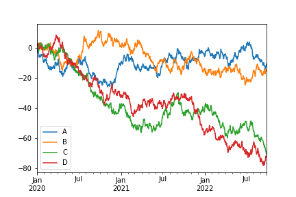
img3.png
11.2 条形图
df = pd.DataFrame({'a': np.random.randn(10) + 1, 'b': np.random.randn(10),
        'c': np.random.randn(10) - 1}, columns=['a', 'b', 'c'])

df['a'].plot.bar()
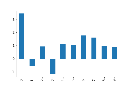
img4.png
调用DataFrame的plot.bar()方法会产生多条图
df = pd.DataFrame({'a': np.random.randn(10) + 1, 'b': np.random.randn(10),
        'c': np.random.randn(10) - 1}, columns=['a', 'b', 'c'])

df.plot.bar()
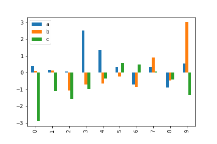
img5.png
要生成堆叠的条形图,传递stacked=True
df.plot.bar(stacked=True)
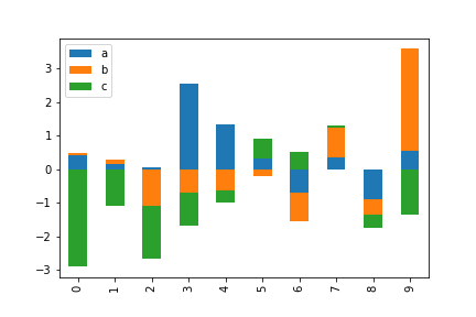
img6.png
要获取水平条形图,使用barh方法
df.plot.barh(stacked=True)
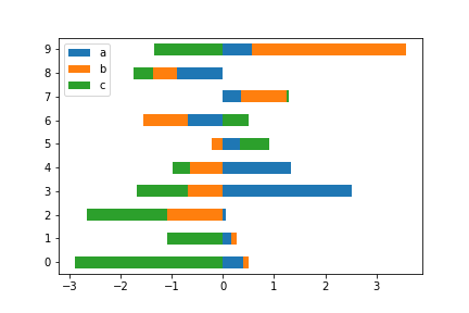
img7.png
11.3 直方图
使用hist()方法绘制直方图
df = pd.DataFrame({'a': np.random.randn(100) + 1, 'b': np.random.randn(100),
        'c': np.random.randn(100) - 1}, columns=['a', 'b', 'c'])

df.plot.hist(alpha=0.8)
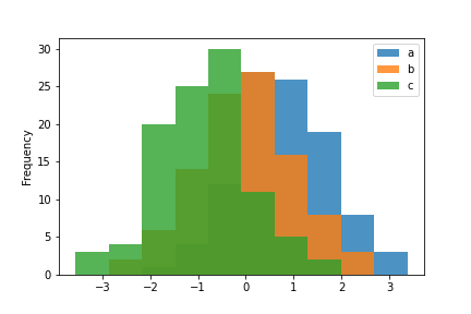
img8.png
同样可以使用stacked=True来堆叠直方图,箱尺寸可以使用bins关键字进行更改
df.plot.hist(stacked=True, bins=30)
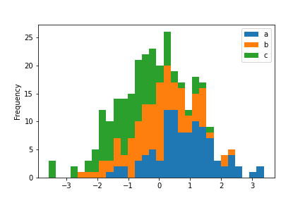
img9.png
可以传递matplotlib支持的其他关键字
df.plot.hist(orientation='horizontal', cumulative=True)
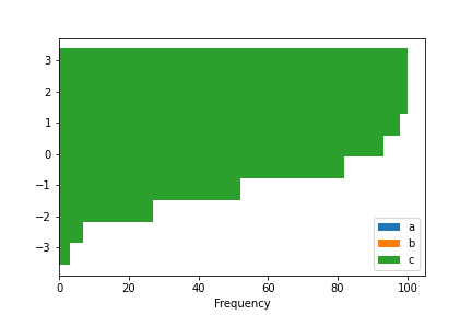
img10.png
绘制多个子图
df = pd.DataFrame({'a': np.random.randn(100) + 1, 'b': np.random.randn(100),
        'c': np.random.randn(100) - 1,'d': np.random.randn(100) * 2}, columns=['a', 'b', 'c', 'd'])

df.hist(color='k', alpha=0.3, bins=30)
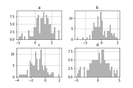
img11.png
11.4 箱型图
可以使用Series.plot.box()和DataFrame.plot.box()绘制箱线图,或者DataFrame.boxplot()可视化每列中值的分布
df = pd.DataFrame(np.random.rand(10, 5), columns=['A', 'B', 'C', 'D', 'E'])

df.plot.box()
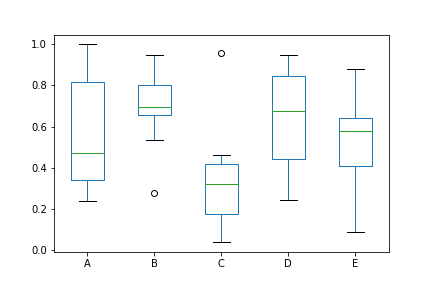
img12.png
可以通过字典传递boxes,whiskers,medians和caps的颜色参数
color = {'boxes': 'DarkGreen', 'whiskers': 'DarkOrange', 'medians': 'DarkBlue', 'caps': 'Gray'}

df.plot.box(color=color, sym='bo')
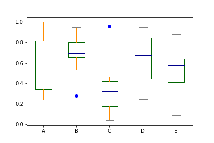
img13.png
图像横置
color = {'boxes': 'DarkGreen', 'whiskers': 'DarkOrange', 'medians': 'DarkBlue', 'caps': 'Gray'}

df.plot.box(color=color, sym='ro', vert=False)
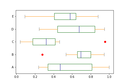
img14.png
使用MatplotLib支持的关键字,例如positions更改坐标轴位置
color = {'boxes': 'DarkGreen', 'whiskers': 'DarkOrange', 'medians': 'DarkBlue', 'caps': 'Gray'}

df.plot.box(color=color, sym='ro', positions=[1, 2, 3, 4, 10])
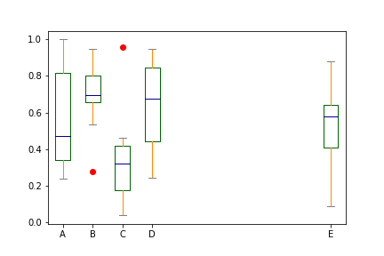
img15.png
DataFrame.boxplot()同样可以用来绘制箱型图
df.boxplot()
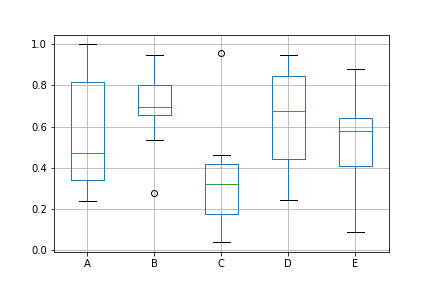
img16.png
根据分组绘制箱型图
df = pd.DataFrame(np.random.randn(10, 2),columns=['Col1', 'Col2'])

df['X'] = pd.Series(['A', 'A', 'A', 'A', 'A', 'B', 'B', 'B', 'B', 'B'])

df.groupby('X').boxplot()
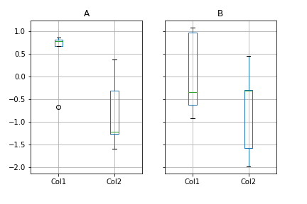
img17.png
11.5 面积图
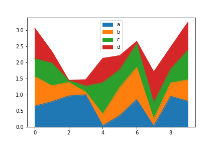
使用area()方法可以绘制面积图
df = pd.DataFrame(np.random.rand(10, 4), columns=['a', 'b', 'c', 'd'])

df.plot.area()
img18.png
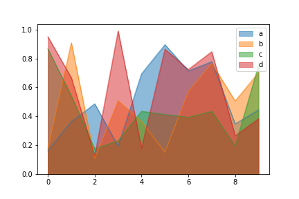
使用stacked=False参数,生成未堆叠的图
df.plot.area(stacked=False)
img19.png
11.6 散点图
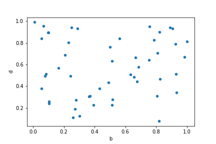
使用scatter()绘制散点图,散点图要求x轴和y轴为数字列,这可以通过关键字指定
df = pd.DataFrame(np.random.rand(50, 4), columns=['a', 'b', 'c', 'd'])

df.plot.scatter(x='b', y='d')
img20.png
要在单个轴上绘制多个列组,可以通过ax方法重复指定plot。但是,最好也指定color和label关键字以区分每个组
ax = df.plot.scatter(x='a', y='b', color='DarkBlue', label='Group 1')

df.plot.scatter(x='c', y='d', color='DarkGreen', label='Group 2', ax=ax)
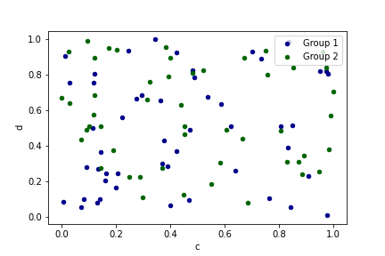
img21.png
关键字c可以作为列的名称来给每个点提供颜色
df.plot.scatter(x='a', y='b', c='r', s=40)
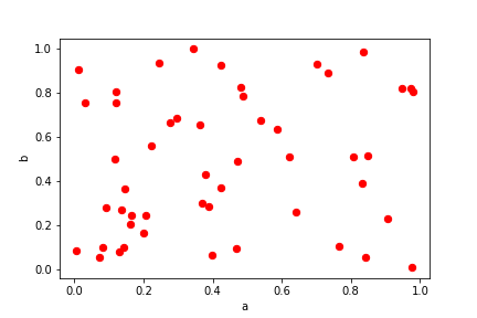
img22.png
关键字s用来指定气泡大小,可以指定DataFrame的列作为参数
df.plot.scatter(x='a', y='b', c='g', s=df['c']*50)
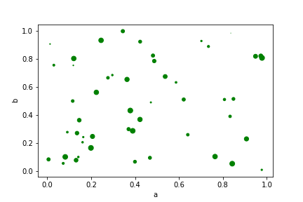
img23.png
11.7 六边形图
如果数据过于密集无法绘制每个点,可以使用六边形图代替散点图。使用hexbin()方法可以绘制六边形图
df = pd.DataFrame(np.random.randn(1000, 2), columns=['a', 'b'])

df['b'] = df['b'] + np.arange(1000)

df.plot.hexbin(x='a', y='b', gridsize=30)
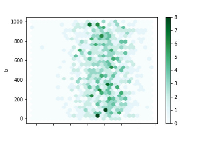
img24.png
关键字参数gridsize控制x方向上六边形的数量,默认为100。
11.8 饼图
使用pie()方法绘制饼图,如果数据包含NaN,会自动填充为0
series = pd.Series(3 * np.random.rand(4), index=['a', 'b', 'c', 'd'], name='series')

series.plot.pie()
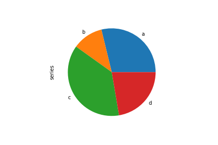
img25.png
对于饼图,最好使用正方形图形,即图形长宽比为1。可以创建宽度和高度相等的图形,或者在绘制后通过调用ax.set_aspect('equal')强制长宽比相等。
在DataFrame中pie()需要通过y指定列
df = pd.DataFrame(3 * np.random.rand(4, 2), index=['a', 'b', 'c', 'd'], columns=['x', 'y'])

df.plot.pie(y=0)
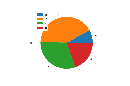
img26.png
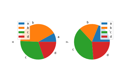
如果不指定具体列,subplots=True可以为每列绘制一个子图
df.plot.pie(subplots=True)
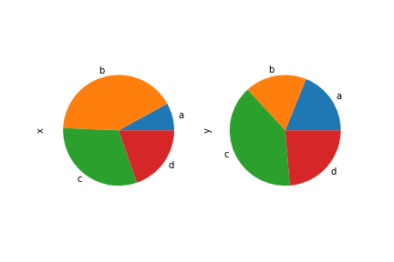
img27.png
如果不想让每个子图都显示图例,用legend=False隐藏它
df.plot.pie(subplots=True, legend=False)
img28.png
MatplotLib的其他参数同样适用
series.plot.pie(labels=['AA', 'BB', 'CC', 'DD'], colors=['r', 'g', 'b', 'c'],autopct='%.2f', fontsize=20, figsize=(6, 6))

img29.png
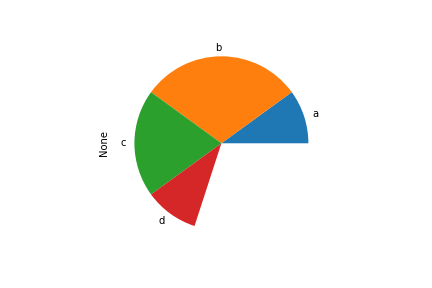
如果数据总和小于1,图形会变成扇形
series = pd.Series([0.1, 0.3, 0.2, 0.1], index=['a', 'b', 'c', 'd'])

series.plot.pie()
img30.png
11.9 缺失数据处理
不同绘图方法对缺失数据的处理方式:
图形 |
NaN处理方式 |
|---|---|
线 |
在NaN处留下空白 |
线(堆叠) |
填0 |
条形图 |
填0 |
散点图 |
丢弃NaN |
直方图 |
删除NaN(按列) |
箱型图 |
删除NaN(按列) |
面积图 |
填0 |
KDE |
删除NaN(按列) |
六边形图 |
丢弃NaN |
饼图 |
填0 |
11.10 散点矩阵
使用 pandas.plotting中的scatter_matrix方法创建散点图矩阵
from pandas.plotting import scatter_matrix

df = pd.DataFrame(np.random.randn(100, 3), columns=['a', 'b', 'c'])

scatter_matrix(df, alpha=0.5)
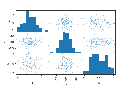
img31.png
11.12 安德鲁斯曲线
安德鲁斯曲线允许将多元数据绘制为大量曲线,这些曲线是使用样本的属性作为傅里叶级数的系数而创建的
from pandas.plotting import andrews_curves

df=pd.DataFrame(np.random.rand(5,10))

df['C'] = pd.Series(['I'+str(x) for x in range(1,6)])

andrews_curves(df, 'C')
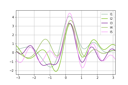
img33.png
11.13 平行坐标
from pandas.plotting import parallel_coordinates

df=pd.DataFrame(np.random.rand(10,10), columns=range(1,11))

df['C'] = pd.Series(['I'+str(x) for x in range(1,6)])

parallel_coordinates(df, 'C')
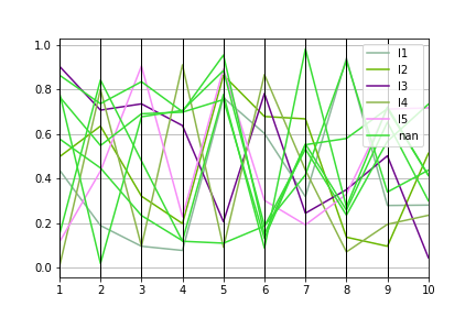
img34.png
11.14 Lag Plot相关性分析
检查数据集或时间序列是否随机。随机数据在滞后图中不应显示任何结构。非随机结构意味着基础数据不是随机的
from pandas.plotting import lag_plot

spacing = np.linspace(-99 * np.pi, 99 * np.pi, num=1000)

data = pd.Series(0.1 * np.random.rand(1000) + 0.9 * np.sin(spacing))

lag_plot(data)
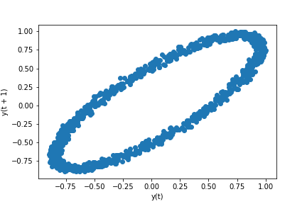
img35.png
11.15 自相关图
自相关图通常用于检查时间序列中的随机性
from pandas.plotting import autocorrelation_plot

spacing = np.linspace(-9 * np.pi, 9 * np.pi, num=1000)

data = pd.Series(0.7 * np.random.rand(1000) + 0.3 * np.sin(spacing))

autocorrelation_plot(data)
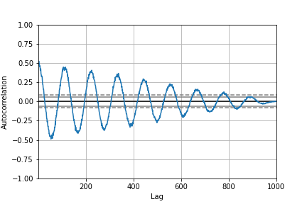
img36.png
11.16 Bootstrap 图
Bootstrap图从数据集中根据指定的次数,重复选择指定大小的随机子集,为该子集计算出相关统计信息。从而可以直观地评估统计数据的不确定性,例如均值,中位数,中间范围等。
from pandas.plotting import bootstrap_plot

data = pd.Series(np.random.rand(1000))

bootstrap_plot(data, size=50, samples=500, color='grey')
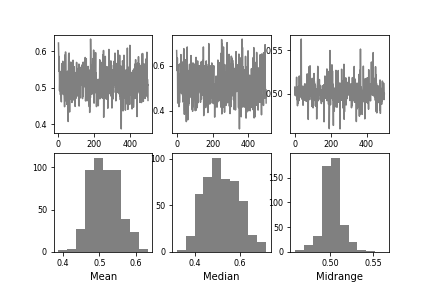
img37.png
11.17 径向坐标
径向坐标可视化是基于弹簧张力最小化算法。它把数据集的特征映射成二维目标空间单位圆中的一个点,点的位置由系在点上的特征决定。把实例投入圆的中心,特征会朝圆中此实例位置(实例对应的归一化数值)“拉”实例。
from pandas.plotting import radviz

df = pd.DataFrame({
            'SepalLength': [6.5, 7.7, 5.1, 5.8, 7.6, 5.0, 5.4, 4.6,
                            6.7, 4.6],
            'SepalWidth': [3.0, 3.8, 3.8, 2.7, 3.0, 2.3, 3.0, 3.2,
                            3.3, 3.6],
            'PetalLength': [5.5, 6.7, 1.9, 5.1, 6.6, 3.3, 4.5, 1.4,
                            5.7, 1.0],
            'PetalWidth': [1.8, 2.2, 0.4, 1.9, 2.1, 1.0, 1.5, 0.2,
                            2.1, 0.2],
            'Category': ['virginica', 'virginica', 'setosa',
                        'virginica', 'virginica', 'versicolor',
                        'versicolor', 'setosa', 'virginica',
                        'setosa']
    })

radviz(df, 'Category')
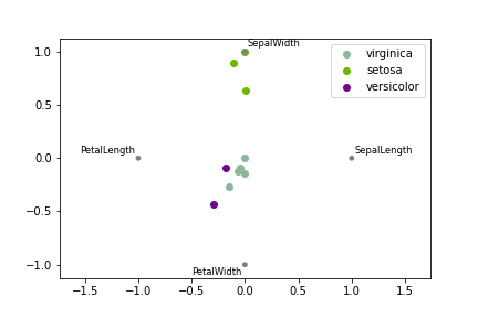
img38.png
11.18 绘图样式
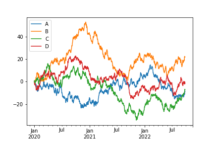
1. 图例
df = pd.DataFrame(np.random.randn(1000, 4),index=ts.index, columns=list('ABCD'))

df = df.cumsum()

df.plot(legend=False)
img39.png
2. 标签
df = pd.DataFrame(np.random.randn(1000, 4),index=ts.index, columns=list('ABCD'))
df = df.cumsum()
ax = df.plot(title = "title: describe figure")
ax.set_xlabel("x label")
ax.set_ylabel("y label")
plt.show()
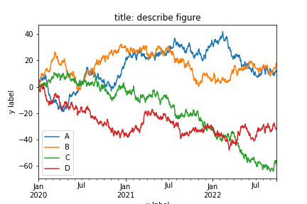
img40.png
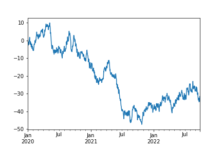
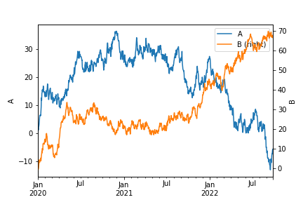
3. 辅助Y轴
df = pd.DataFrame(np.random.randn(1000, 4),index=ts.index, columns=list('ABCD'))
df = df.cumsum()
df['A'].plot(legend=True)
df['B'].plot(secondary_y=True,legend=True)
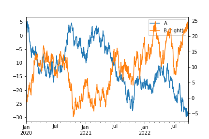
img41.png
设置辅助轴标签
df = pd.DataFrame(np.random.randn(1000, 4),index=ts.index, columns=list('ABCD'))
df = df.cumsum()
ax=df['A'].plot(legend=True)
df['B'].plot(secondary_y=True,legend=True)

ax.set_ylabel("A")
ax.right_ax.set_ylabel("B")
img42.png
使用 mark_right=False可以取消图例中的right标志
ax=df['A'].plot(legend=True)
df['B'].plot(secondary_y=True,legend=True,mark_right=False)

ax.set_ylabel("A")
ax.right_ax.set_ylabel("B")

img43.png
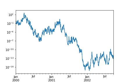
4. 指数刻度
ts = pd.Series(np.random.randn(1000), index=pd.date_range('1/1/2000', periods=1000))
ts = np.exp(ts.cumsum())
ts.plot(logy=True)
img44.png
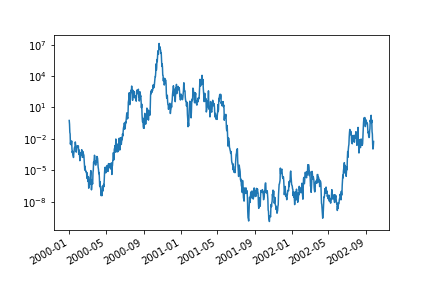
5. 取消时间轴刻度调整
ts.plot(logy=True, x_compat=True)
img45.png
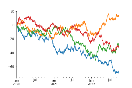
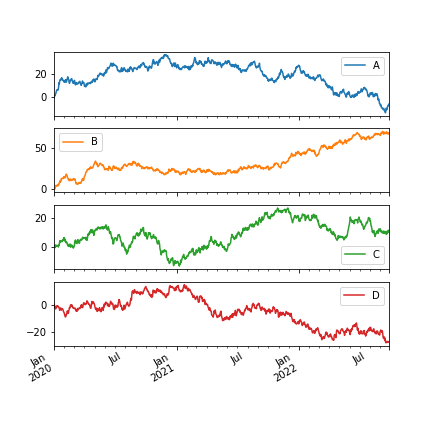
多个视图
with pd.plotting.plot_params.use('x_compat', True):
                df['A'].plot(color='r')
                df['B'].plot(color='g')
                df['C'].plot(color='b')
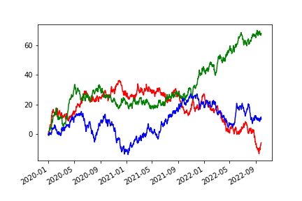
img46.png
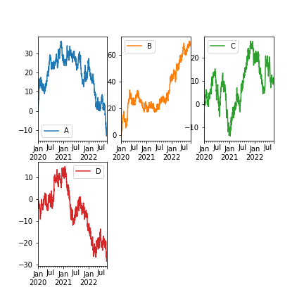
7. 布局定位多个图
df.plot(subplots=True, layout=(2, 3), figsize=(6, 6), sharex=False)
img48.png
也可以通过ax关键字以列表形式传递预先创建的多个轴
fig, axes = plt.subplots(4, 4, figsize=(9, 9))
plt.subplots_adjust(wspace=0.5, hspace=0.5)
target1 = [axes[0][0], axes[1][1], axes[2][2], axes[3][3]]
target2 = [axes[3][0], axes[2][1], axes[1][2], axes[0][3]]
df.plot(subplots=True, ax=target1, legend=False, sharex=False, sharey=False)
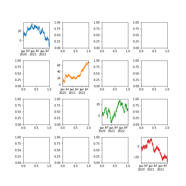
img49.png
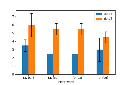
8. 误差线
ix = pd.MultiIndex.from_arrays([['a', 'a', 'a', 'a', 'b', 'b', 'b', 'b'],
                                 ['foo', 'foo', 'bar', 'bar', 'foo', 'foo', 'bar', 'bar']],
                                names=['letter', 'word'])
df = pd.DataFrame({'data1': [3, 2, 4, 3, 2, 4, 3, 2],
                    'data2': [6, 5, 7, 5, 4, 5, 6, 5]}, index=ix)
gp = df.groupby(level=('letter', 'word'))
means = gp.mean()
errors = gp.std()

means

        d       ata1    data2
letter  word
a       bar     3.5     6.0
        foo     2.5     5.5
b       bar     2.5     5.5
        foo     3.0     4.5

errors

                data1       data2
letter  word
a       bar     0.707107    1.414214
        foo     0.707107    0.707107
b       bar     0.707107    0.707107
        foo     1.414214    0.707107

means.plot.bar(yerr=errors, ax=ax, capsize=4, rot=0)    # capsize 控制误差线两端宽度
img50.png
9. 绘制表格
绘制表格的简单方法是指定table=True
df = pd.DataFrame(np.random.randn(4, 4), columns=list('ABCD'))
fig, ax = plt.subplots(1, 1, figsize=(7, 6.5))
ax.xaxis.tick_top() # x轴刻度置于顶部
df.plot(table=True, ax=ax)
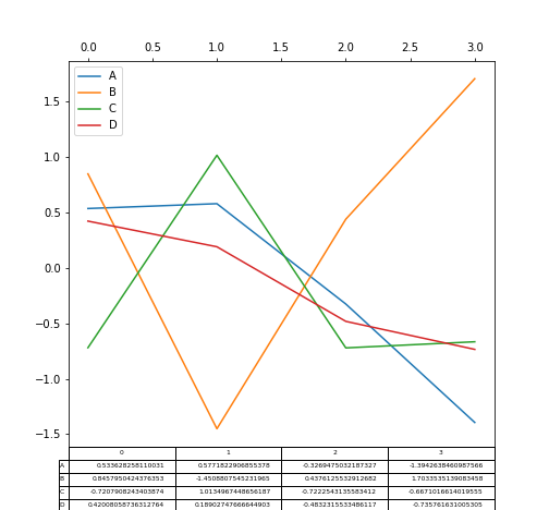
img51.png